Probability Concepts

This topic review covers important terms and concepts associated with probability theory. Random variables, events, outcomes, conditional probability, and joint probability are described. Probability rules such as the addition rule and multiplication rule are introduced. These rules are frequently used by finance practitioners. Expected value, standard deviation, covariance, and correlation for individual asset and portfolio returns are discussed. A well-prepared candidate will be able to calculate and interpret these widely used measures. This review also discusses counting rules, which lay the foundation for the binomial probability distribution that is covered in the next topic review.

1: CONDITIONAL AND JOINT PROBABILITIES

A: Define a random variable, an outcome, an event, mutually exclusive events, and exhaustive events.

• A random variable is an uncertain quantity/number.
• An outcome is an observed value of a random variable.
• An event is a single outcome or a set of outcomes.
• Mutually exclusive events are events that cannot both happen at the same time.
• Exhaustive events are those that include all possible outcomes.

Consider rolling a 6-sided die. The number that comes up is a random variable. If you roll a 4, that is an outcome. Rolling a 4 is an event, and rolling an even number is an event. Rolling a 4 and rolling a 6 are mutually exclusive events. Rolling an even number and rolling an odd number is a set of mutually exclusive and exhaustive events.

B: State the two defining properties of probability and distinguish among empirical, subjective, and a priori probabilities.

There are two defining properties of probability.

• The probability of occurrence of any event ($E_i$) is between 0 and 1 (i.e., $0 \leq P(E_i) \leq 1$).
• If a set of events, $E_1, E_2, \ldots, E_n$, is mutually exclusive and exhaustive, the probabilities of those events sum to 1 (i.e., $\sum P(E_i) = 1$).

The first of the defining properties introduces the term $P(E_i)$, which is shorthand for the “probability of event i.” If $P(E_i) = 0$, the event will never happen. If $P(E_i) = 1$, the event is certain to occur, and the outcome is not random.

The probability of rolling any one of the numbers 1–6 with a fair die is $1/6 = 0.1667 = 16.7\%$. The set of events—rolling a number equal to 1, 2, 3, 4, 5, or 6—is exhaustive, and the individual events are mutually exclusive, so the probability of this set of events is equal to 1. We are certain that one of the values in this set of events will occur.

An empirical probability is established by analyzing past data. An a priori probability is determined using a formal reasoning and inspection process. A subjective probability is the least formal method of developing probabilities and involves the use of personal judgment. An analyst may know many things about a firm’s performance and have expectations about the overall market that are all used to arrive at a subjective probability, such as, “I believe there is a 70% probability that Acme Foods will outperform the market this year.” Empirical and a priori probabilities, by contrast, are objective probabilities.

C: State the probability of an event in terms of odds for and against the event.

Stating the odds that an event will or will not occur is an alternative way of expressing probabilities. Consider an event that has a probability of occurrence of 0.125, which is one-eighth. The odds that the event will occur are $\frac{0.125}{(1 - 0.125)} = \frac{1/8}{7/8} = \frac{1}{7}$, which we state as, “the odds for the event occurring are one-to-seven.” The odds against the event occurring are the reciprocal of $1/7$, which is seven-to-one.

We can also get the probability of an event from the odds by reversing these calculations. If we know that the odds for an event are one-to-six, we can compute the probability of occurrence as $\frac{1}{1+6} = \frac{1}{7} = 0.1429 = 14.29\%$. Alternatively, the probability that the event will not occur is $\frac{6}{1+6} = \frac{6}{7} = 0.8571 = 85.71\%$.

PROFESSOR’S NOTE

While I am quite familiar with the use of odds rather than probabilities at the horse track, I can’t remember encountering odds for a stock or bond. The use of odds at the horse track lets you know how much you will win per $1 bet on a horse (less the track’s percentage). If you bet on a 15-1 long shot and the horse wins, you will receive $15 and your $1 bet will be returned, so the profit is $15. Of course, if the horse loses, you would lose the $1 you bet and the “profit” is -$1.

One last point is that the expected return on the bet is zero, based on the probability of winning expressed in the odds. The probability of the horse winning when the odds are 15-to-1 is $\frac{1}{15+1} = \frac{1}{16}$ and the probability of the horse losing is $15/16$. The expected profit is $\frac{1}{16} \times \$15 + \frac{15}{16} \times (-\$1) = 0$.

D: Distinguish between unconditional and conditional probabilities.

• Unconditional probability (a.k.a. marginal probability) refers to the probability of an event regardless of the past or future occurrence of other events. If we are concerned with the probability of an economic recession, regardless of the occurrence of changes in interest rates or inflation, we are concerned with the unconditional probability of a recession.

• A conditional probability is one where the occurrence of one event affects the probability of the occurrence of another event. For example, we might be concerned with the probability of a recession given that the monetary authority increases interest rates. This is a conditional probability. The key word to watch for here is “given.” Using probability notation, “the probability of A given the occurrence of B” is expressed as $P(A | B)$, where the vertical bar ($|$) indicates “given,” or “conditional upon.” For our interest rate example above, the probability of a recession given an increase in interest rates is expressed as $P(\text{recession}\ | \ \text{increase in interest rates})$. A conditional probability of an occurrence is also called its likelihood.

E: Explain the multiplication, addition, and total probability rules.

The multiplication rule of probability is used to determine the joint probability of two events:

$$P(AB) = P(A \mid B) \times P(B)$$

The addition rule of probability is used to determine the probability that at least one of two events will occur:

$$P(A \text{ or } B) = P(A) + P(B) - P(AB)$$

The total probability rule is used to determine the unconditional probability of an event, given conditional probabilities:

$$P(A) = P(A \mid B_1)P(B_1) + P(A \mid B_2)P(B_2) + \ldots + P(A \mid B_N)P(B_N)$$

where $B_1, B_2, \ldots B_N$ is a mutually exclusive and exhaustive set of outcomes.

F: Calculate and interpret 1) the joint probability of two events, 2) the probability that at least one of two events will occur, given the probability of each and the joint probability of the two events, and 3) a joint probability of any number of independent events.

The joint probability of two events is the probability that they will both occur. We can calculate this from the conditional probability that A will occur given B occurs (a conditional probability) and the probability that B will occur (the unconditional probability of B). This calculation is sometimes referred to as the multiplication rule of probability. Using the notation for conditional and unconditional probabilities we can express this rule as:

$$P(AB) = P(A | B) \times P(B)$$

This expression is read as follows: “The joint probability of A and B, $P(AB)$, is equal to the conditional probability of A given B, $P(A | B)$, times the unconditional probability of B, $P(B)$.”

This relationship can be rearranged to define the conditional probability of A given B as follows:

$$P(A|B) = \frac{P(AB)}{P(B)}$$

EXAMPLE: Multiplication rule of probability

Consider the following information:

• P(I) = 0.4, the probability of the monetary authority increasing interest rates (I) is 40%.
• P(R | I) = 0.7, the probability of a recession (R) given an increase in interest rates is 70%.

What is P(RI), the joint probability of a recession and an increase in interest rates?

Answer:

Applying the multiplication rule, we get the following result:

$$\begin{align*} P(RI) &= P(R | I) \times P(I) \\ P(RI) &= 0.7 \times 0.4 \\ P(RI) &= 0.28 \end{align*}$$

Don’t let the cumbersome notation obscure the simple logic of this result. If an interest rate increase will occur 40% of the time and lead to a recession 70% of the time when it occurs, the joint probability of an interest rate increase and a resulting recession is (0.4)(0.7) = (0.28) = 28%.

Calculating the Probability That at Least One of Two Events Will Occur

The addition rule for probabilities is used to determine the probability that at least one of two events will occur. For example, given two events, A and B, the addition rule can be used to determine the probability that either A or B will occur. If the events are not mutually exclusive, double counting must be avoided by subtracting the joint probability that both A and B will occur from the sum of the unconditional probabilities. This is reflected in the following general expression for the addition rule:

$$P(A \text{ or } B) = P(A) + P(B) - P(AB)$$

For mutually exclusive events, where the joint probability, $P(AB)$, is zero, the probability that either A or B will occur is simply the sum of the unconditional probabilities for each event, $P(A \text{ or } B) = P(A) + P(B)$.

Figure: Venn Diagram for Events That Are Not Mutually Exclusive

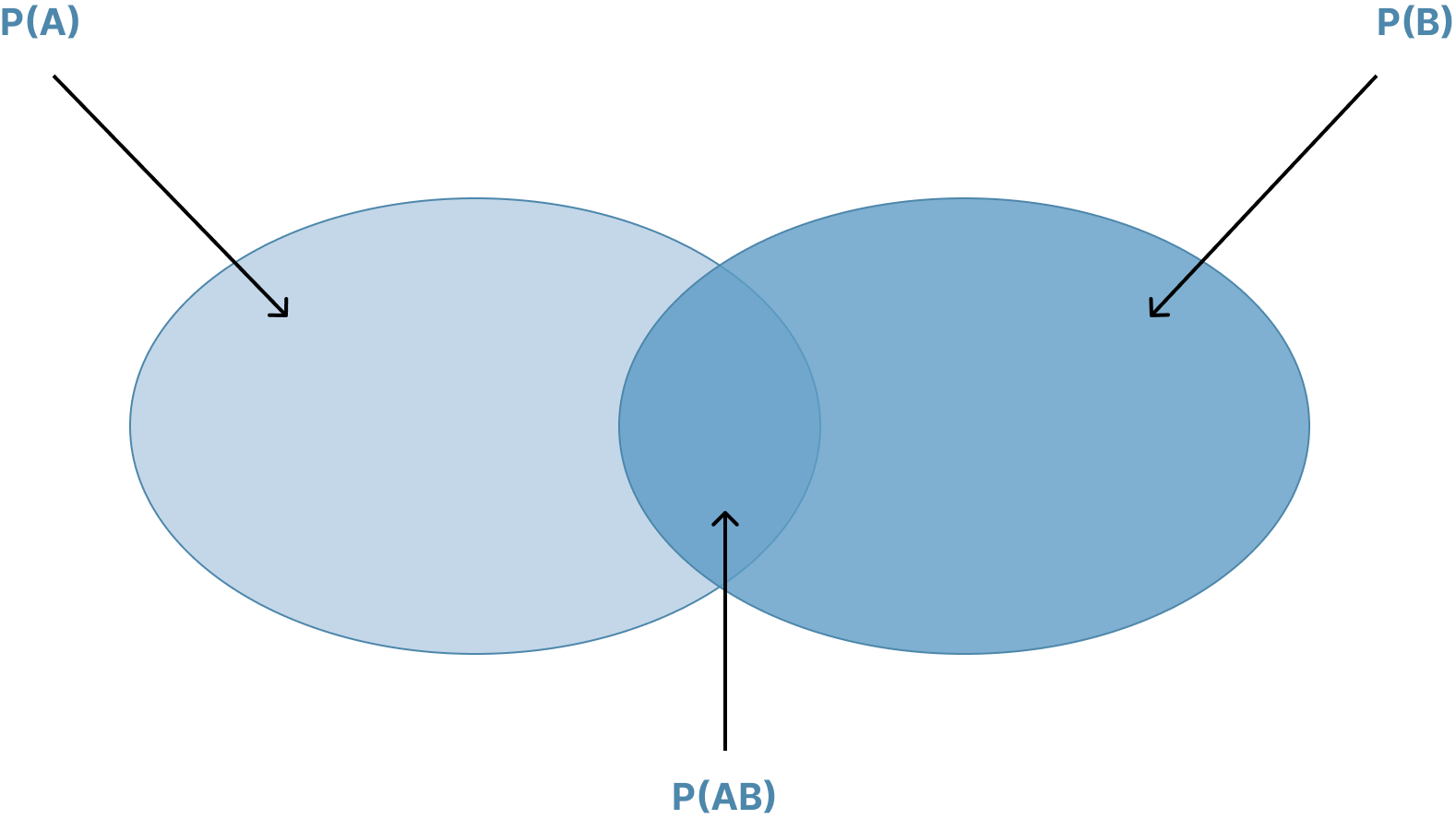
The figure illustrates the addition rule with a Venn Diagram and highlights why the joint probability must be subtracted from the sum of the unconditional probabilities. Note that if the events are mutually exclusive the sets do not intersect, $P(AB) = 0$, and the probability that one of the two events will occur is simply $P(A) + P(B)$.

EXAMPLE: Addition rule of probability

Using the information in our previous interest rate and recession example and the fact that the unconditional probability of a recession, $P(R)$, is 34%, determine the probability that either interest rates will increase or a recession will occur.

Answer: Given that $P(R) = 0.34$, $P(I) = 0.40$, and $P(RI) = 0.28$, we can compute $P(R \text{ or } I)$ as follows:

$$P(R \text{ or } I) = P(R) + P(I) - P(RI)$$$$P(R \text{ or } I) = 0.34 + 0.40 - 0.28$$$$P(R \text{ or } I) = 0.46$$

Calculating a Joint Probability of any Number of Independent Events

On the roll of two dice, the joint probability of getting two 4s is calculated as:

$$P(4 \text{ on first die and 4 on second die}) = P(4 \text{ on first die}) \times P(4 \text{ on second die}) = \frac{1}{6} \times \frac{1}{6} = \frac{1}{36} = 0.0278$$

On the flip of two coins, the probability of getting two heads is:

$$P(\text{heads on first coin and heads on second coin}) = \frac{1}{2} \times \frac{1}{2} = \frac{1}{4} = 0.25$$

Hint: When dealing with independent events, the word and indicates multiplication, and the word or indicates addition. In probability notation:

$$P(A \textbf{ or } B) = P(A) + P(B) - P(AB), \text{ and } P(A \textbf{ and } B) = P(A) \times P(B)$$

The multiplication rule we used to calculate the joint probability of two independent events may be applied to any number of independent events, as the following example illustrates.

EXAMPLE: Joint probability for more than two independent events

What is the probability of rolling three 4s in one simultaneous toss of three dice?

Answer: Since the probability of rolling a 4 for each die is 1/6, the probability of rolling three 4s is:

$$P(\text{three 4s on the roll of three dice}) = \frac{1}{6} \times \frac{1}{6} \times \frac{1}{6} = \frac{1}{216} = 0.00463$$

📝 QUIZ

1. An event that includes all of the possible outcomes is said to be:

• A. random.
• B. exclusive.
• C. exhaustive.

2. Which of the following values cannot be the probability of an event?

• A. 0.00.
• B. 1.00.
• C. 1.25.

3. The probability that the DJIA will increase tomorrow is 2/3. The probability of an increase in the DJIA stated as odds is:

• A. two-to-one.
• B. one-to-three.
• C. two-to-three.

4. The multiplication rule of probability determines the joint probability of two events as the product of:

• A. two conditional probabilities.
• B. two unconditional probabilities.
• C. a conditional probability and an unconditional probability.

5. If events A and B are mutually exclusive, then:

• A. P(A | B) = P(A).
• B. P(AB) = P(A) x P(B).
• C. P(A or B) = P(A) + P(B).

6. At a charity ball, 800 names are put into a hat. Four of the names are identical. On a random draw, what is the probability that one of these four names will be drawn?

• A. 0.004.
• B. 0.005.
• C. 0.010.

7. Two mutually exclusive events:

• A. always occur together.
• B. cannot occur together.
• C. can sometimes occur together.

2: CONDITIONAL EXPECTATIONS, CORRELATION

G: Distinguish between dependent and independent events.

Independent events refer to events for which the occurrence of one has no influence on the occurrence of the others. The definition of independent events can be expressed in terms of conditional probabilities. Events A and B are independent if and only if:

$$P(A | B) = P(A), \text{ or equivalently, } P(B | A) = P(B)$$

If this condition is not satisfied, the events are dependent events (i.e., the occurrence of one is dependent on the occurrence of the other).

In our interest rate and recession example, recall that events I and R are not independent; the occurrence of I affects the probability of the occurrence of R. In this example, the independence conditions for I and R are violated because:

$$P(R) = 0.34, \text{ but } P(R | I) = 0.7;$$

the probability of a recession is greater when there is an increase in interest rates.

The best examples of independent events are found with the a priori probabilities of dice tosses or coin flips. A die has “no memory.” Therefore, the event of rolling a 4 on the second toss is independent of rolling a 4 on the first toss. This idea may be expressed as:

$$P(4 \text{ on second toss } | 4 \text{ on first toss }) = P(4 \text{ on second toss }) = 1/6 \text{ or } 0.167$$

The idea of independent events also applies to flips of a coin:

$$P(\text{heads on first coin } | \text{ heads on second coin}) = P(\text{heads on first coin}) = 1/2 \text{ or } 0.50$$

H: Calculate and interpret an unconditional probability using the total probability rule.

The total probability rule highlights the relationship between unconditional and conditional probabilities of mutually exclusive and exhaustive events. It is used to explain the unconditional probability of an event in terms of probabilities that are conditional upon other events.

In general, the unconditional probability of event R,

$$P(R) = P(R | S_1) × P(S_1) + P(R | S_2) × P(S_2) + . . . + P(R | S_N) × P(S_N)$$

where the set of events ${S_1, S_2, . . . S_N}$ is mutually exclusive and exhaustive.

EXAMPLE: An investment application of unconditional probability

Building upon our ongoing example about interest rates and economic recession, we can assume that a recession can only occur with either of the two events—interest rates increase (I) or interest rates do not increase ($I^C$)—since these events are mutually exclusive and exhaustive. $I^C$ is read "the complement of I," which means "not I." Therefore, the probability of $I^C$ is $1 - P(I)$. It is logical, therefore, that the sum of the two joint probabilities must be the unconditional probability of a recession. This can be expressed as follows:

$$P(R) = P(RI) + P(RI^C)$$

Applying the multiplication rule, we may restate this expression as:

$$P(R) = P(R | I) × P(I) + P(R | I^C) × P(I^C)$$

Assume that $P(R | I) = 0.70, P(R | I^C)$, the probability of recession if interest rates do not rise, is 10% and that $P(I) = 0.40$ so that $P(I^C) = 0.60$. The unconditional probability of a recession can be calculated as follows:

$$P(R) = P(R | I) × P(I) + P(R | I) × P(I) \\ = (0.70)(0.40) + (0.10)(0.60) \\ = 0.28 + 0.06 = 0.34$$

Expected Value

The expected value of a random variable is the weighted average of the possible outcomes for the variable. The mathematical representation for the expected value of random variable (X) is:

$$E(X) = \Sigma P(x_i)x_i = P(x_1)x_1 + P(x_2)x_2 + \cdots + P(x_n)x_n$$

EXAMPLE: Expected earnings per share

The probability distribution of EPS for Ron’s Stores is given in the figure below. Calculate the expected earnings per share.

EPS Probability Distribution

Probability	Earnings Per Share
10%	£1.80
20%	£1.60
40%	£1.20
30%	£1.00

Answer:

The expected EPS is simply a weighted average of each possible EPS, where the weights are the probabilities of each possible outcome.

$$E[\text{EPS}] = 0.10(1.80) + 0.20(1.60) + 0.40(1.20) + 0.30(1.00) = £1.28$$

I: Explain the use of conditional expectation in investment applications.

Expected values or returns can be calculated using conditional probabilities. As the name implies, conditional expected values are contingent upon the outcome of some other event. An analyst would use a conditional expected value to revise his expectations when new information arrives.

Consider the effect of a tariff on steel imports on the returns of a domestic steel stock. The stock’s expected return, given that the government imposes the tariff, will be higher than the expected return if the tariff is not imposed.

Using the total probability rule, we can estimate the (unconditional) expected return on the stock as the sum of the expected return given no tariff times the probability a tariff will not be enacted plus the expected return given a tariff times the probability a tariff will be enacted.

J: Explain the use of a tree diagram to represent an investment problem.

You might well wonder where the returns and probabilities used in calculating expected values come from. A general framework called a tree diagram is used to show the probabilities of various outcomes. In the following figure, we have shown estimates of EPS for four different outcomes: (1) a good economy and relatively good results at the company, (2) a good economy and relatively poor results at the company, (3) a poor economy and relatively good results at the company, and (4) a poor economy and relatively poor results at the company. Using the rules of probability, we can calculate the probabilities of each of the four EPS outcomes shown in the boxes on the right-hand side of the “tree.”

The expected EPS of $1.51 is simply calculated as:

$$0.18 \times 1.80 + 0.42 \times 1.70 + 0.24 \times 1.30 + 0.16 \times 1.00 = \$1.51$$

Note that the probabilities of the four possible outcomes sum to 1.

Figure: A Tree Diagram

K: Calculate and interpret covariance and correlation and interpret a scatterplot.

The variance and standard deviation measure the dispersion, or volatility, of only one variable. In many finance situations, however, we are interested in how two random variables move in relation to each other. For investment applications, one of the most frequently analyzed pairs of random variables is the returns of two assets. Investors and managers frequently ask questions such as, “what is the relationship between the return for Stock A and Stock B?” or, “what is the relationship between the performance of the S&P 500 and that of the automotive industry?”

Covariance is a measure of how two assets move together. It is the expected value of the product of the deviations of the two random variables from their respective expected values. A common symbol for the covariance between random variables X and Y is Cov(X, Y). Since we will be mostly concerned with the covariance of asset returns, the following formula has been written in terms of the covariance of the return of asset i, $R_i$, and the return of asset j, $R_j$:

$$\text{Cov}(R_i, R_j) = \mathrm{E}[(R_i - \mathrm{E}(R_i))(R_j - \mathrm{E}(R_j))]$$

The following are properties of the covariance:

• The covariance is a general representation of the same concept as the variance. That is, the variance measures how a random variable moves with itself, and the covariance measures how one random variable moves with another random variable.
• The covariance of $R_A$ with itself is equal to the variance of $R_A$; that is, $\text{Cov}(R_A, R_A) = \text{Var}(R_A)$.
• The covariance may range from negative infinity to positive infinity.

To aid in the interpretation of covariance, consider the returns of a stock and of a put option on the stock. These two returns will have a negative covariance because they move in opposite directions. The returns of two automotive stocks would likely have a positive covariance, and the returns of a stock and a riskless asset would have a zero covariance because the riskless asset’s returns never move, regardless of movements in the stock’s return. While the formula for covariance given previously is correct, the method of computing the covariance of returns from a joint probability model uses a probability-weighted average of the products of the random variable’s deviations from their means for each possible outcome. The following example illustrates this calculation.

EXAMPLE: Covariance

Assume that the economy can be in three possible states (S) next year: boom, normal, or slow economic growth. An expert source has calculated that $P(boom) = 0.30, P(normal) = 0.50,\ \text{and}\ P(slow) = 0.20$. The returns for Stock A, $R_A$, and Stock B, $R_B$, under each of the economic states are provided in the probability model as follows. What is the covariance of the returns for Stock A and Stock B?

Probability Distribution of Returns

Event	P(S)	$R_A$	$R_B$
Boom	0.3	0.20	0.30
Normal	0.5	0.12	0.10
Slow	0.2	0.05	0.00

Answer:

First, the expected returns for each of the stocks must be determined.

$$E(R_A) = (0.3)(0.20) + (0.5)(0.12) + (0.2)(0.05) = 0.13$$$$E(R_B) = (0.3)(0.30) + (0.5)(0.10) + (0.2)(0.00) = 0.14$$

The covariance can now be computed using the procedure described in the following table.

Covariance Computation

Event	P(S)	$R_A$	$R_B$	$P(S) \times [R_A - E(R_A)] \times [R_B - E(R_B)]$
Boom	0.3	0.20	0.30	$(0.3)(0.2 - 0.13)(0.3 - 0.14) = 0.00336$
Normal	0.5	0.12	0.10	$(0.5)(0.12 - 0.13)(0.1 - 0.14) = 0.00020$
Slow	0.2	0.05	0.00	$(0.2)(0.05 - 0.13)(0 - 0.14) = 0.00224$

$$\text{Cov}(R_A, R_B) = \sum \{ P(S) \times [R_A - E(R_A)] \times [R_B - E(R_B)] \} = 0.00580$$

So far, we have calculated covariance from a probability model. We can also determine covariance using historical data. The calculation of the sample covariance is based on the following formula:

$$\text{Cov}_{1,2} = \frac{\sum_{t=1}^{n}\{(R_{t,1} - \overline{R_1})(R_{t,2} - \overline{R_2})\}}{n-1}$$

where:

• $R_{t,1}$ = return on Asset 1 in period $t$
• $R_{t,2}$ = return on Asset 2 in period $t$
• $\overline{R_1}$ = mean return on Asset 1
• $\overline{R_2}$ = mean return on Asset 2
• $n$ = number of periods

In practice, the covariance is difficult to interpret. This is mostly because it can take on extremely large values, ranging from negative to positive infinity, and, like the variance, these values are expressed in terms of square units.

To make the covariance of two random variables easier to interpret, it may be divided by the product of the random variables’ standard deviations. The resulting value is called the correlation coefficient, or simply, correlation. The relationship between covariances, standard deviations, and correlations can be seen in the following expression for the correlation of the returns for asset $i$ and $j$:

$$\text{Corr} (R_i, R_j) = \frac{\text{Cov}(R_i, R_j)}{\sigma (R_i) \sigma (R_j)}$$

which implies

$$\text{Cov}(R_i, R_j) = \text{Corr} (R_i, R_j) \sigma (R_i) \sigma (R_j)$$

The correlation between two random return variables may also be expressed as $\rho(R_i,R_j)$, or $\rho_{i,j}$. Correlation can be forward-looking if it uses covariance from a probability model, or backward-looking if it uses sample covariance from historical data.

Properties of correlation of two random variables $R_i$ and $R_j$ are summarized here:

• Correlation measures the strength of the linear relationship between two random variables.
• Correlation has no units.
• The correlation ranges from $-1$ to $+1$. That is, $-1 \leq \text{Corr}(R_i, R_j) \leq +1$.
• If $\text{Corr}(R_i, R_j) = 1.0$, the random variables have perfect positive correlation. This means that a movement in one random variable results in a proportional positive movement in the other relative to its mean.
• If $\text{Corr}(R_i, R_j) = -1.0$, the random variables have perfect negative correlation. This means that a movement in one random variable results in an exact opposite proportional movement in the other relative to its mean.
• If $\text{Corr}(R_i, R_j) = 0$, there is no linear relationship between the variables, indicating that prediction of $R_i$ cannot be made on the basis of $R_j$ using linear methods.

EXAMPLE: Correlation

Using our previous example, compute and interpret the correlation of the returns for stocks A and B, given that $\sigma^2(R_A) = 0.0028$ and $\sigma^2(R_B) = 0.0124$ and recalling that $\text{Cov}(R_A, R_B) = 0.0058$.

Answer:

First, it is necessary to convert the variances to standard deviations.

$$\sigma(R_A) = (0.0028)^{\frac{1}{2}} = 0.0529$$$$\sigma(R_B) = (0.0124)^{\frac{1}{2}} = 0.1114$$

Now, the correlation between the returns of Stock A and Stock B can be computed as follows:

$$\text{Corr}(R_A, R_B) = \frac{0.0058}{(0.0529)(0.1114)} = 0.9842$$

The fact that this value is close to +1 indicates that the linear relationship is not only positive but very strong.

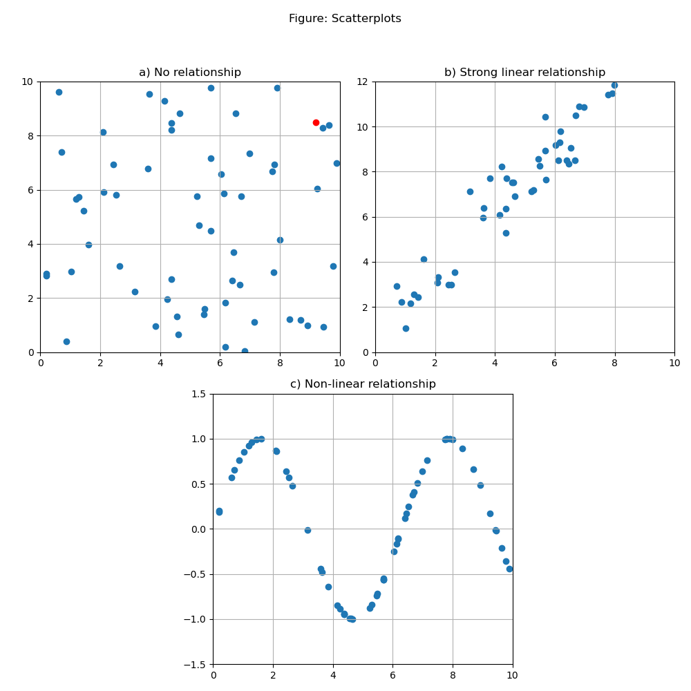
Scatterplots are a method for displaying the relationship between two variables. With one variable on the vertical axis and the other on the horizontal axis, their paired observations can each be plotted as a single point. For example, in panel a of the following figure, there is a red point showing that when one of the variables (on the horizontal axis) is 9.2, the other variable (on the vertical axis) is 8.5.

The scatterplot in panel a is typical of two variables that have no clear relationship. Panel b shows two variables that have a strong linear relationship, that is, a high correlation coefficient.

A key advantage of creating scatterplots is that they can reveal non-linear relationships, which are not described by the correlation coefficient. Panel c illustrates such a relationship. Although the correlation coefficient for these two variables is close to zero, their scatterplot shows clearly that they are related in a predictable way.

Care should be taken when drawing conclusions based on correlation. Causation isn’t implied just from significant correlation. Even if it were, which variable is “causing” change in the other isn’t revealed by correlation. It is more prudent to say that two variables exhibit positive (or negative) association, suggesting that the nature of any causal relationship is to be separately investigated or based on theory that can be subject to additional tests.

One question that can be investigated is the role of outliers (extreme values) in the correlation of two variables. If removing the outliers significantly reduces the calculated correlation, further inquiry is necessary into whether the outliers provide information or are caused by noise (randomness) in the data used.

Spurious correlation refers to correlation that is either the result of chance or present due to changes in both variables over time that is caused by their association with a third variable.

For example, we can find instances where two variables that are both related to the inflation rate exhibit significant correlation, but for which causation in either direction is not the case.

In his book Spurious Correlation, Tyler Vigen presents the following examples. The correlation between the age of each year’s Miss America and the number of films Nicholas Cage appeared in that year is 87%. This seems a bit random. The correlation between the U.S. spending on science, space, and technology and suicides by hanging, strangulation, and suffocation over the 1999–2009 period is 99.87%. Impressive correlation, but both variables increased in an approximately linear fashion over the period.

PROFESSOR’S NOTE

Here, the passage of time seems to be the “third variable” driving the results. Why, I have no idea, but I’m 99.87% sure that neither of the two variables is the cause of the other.

📝 QUIZ

1. Two events are said to be independent if the occurrence of one event:

• A. means that the second event cannot occur.
• B. means that the second event is certain to occur.
• C. does not affect the probability of the occurrence of the other event.

2. An analyst estimates that a share price has an 80% probability of increasing if economic growth exceeds 3%, a 40% probability of increasing if economic growth is positive but less than 3%, and a 10% probability of increasing if economic growth is negative. If economic growth has a 25% probability of exceeding 3% and a 25% probability of being negative, what is the probability that the share price increases?

• A. 22.5%
• B. 42.5%
• C. 62.5%

3. Possible values for the covariance of two random variables are:

• A. unbounded.
• B. bounded by 0 and 1.
• C. bounded by –1 and 1.

PORTFOLIO VARIANCE, BAYES, AND COUNTING PROBLEMS

L: Calculate and interpret the expected value, variance, and standard deviation of a random variable and of returns on a portfolio.

Recall that the expected value of a random variable is the weighted average of its possible outcomes:

$$E(X) = \Sigma P(x_i)x_i = P(x_1)x_1 + P(x_2)x_2 + \ldots + P(x_n)x_n$$

The expected value and variance for a portfolio of assets can be determined using the properties of the individual assets in the portfolio. To do this, it is necessary to establish the portfolio weight for each asset. As indicated in the formula, the weight, $w$, of portfolio asset $i$ is simply the market value currently invested in the asset divided by the current market value of the entire portfolio.

$$w_i = \frac{\text{market value of investment in asset } i}{\text{market value of the portfolio}}$$

Portfolio expected value. The expected value of a portfolio composed of $n$ assets with weights, $w_i$, and expected values, $R_i$, can be determined using the following formula:

$$E(R_p) = \sum_{i=1}^{N} w_i E(R_i) = w_1 E(R_1) + w_2 E(R_2) + \ldots + w_n E(R_n)$$

More often, we have expected returns (rather than expected prices). When the $R_i$ are returns, the expected return for a portfolio, $E(R_p)$, is calculated using the asset weights and the same formula as above.

Portfolio variance. The variance of the portfolio return uses the portfolio weights also, but in a more complicated way:

$$\text{Var}(R_p) = \sum_{i=1}^{N} \sum_{j=1}^{N} w_i w_j \text{Cov}(R_i, R_j)$$

The variance of a portfolio composed of risky asset $A$ and risky asset $B$ can be expressed as:

$$\text{Var}(R_p) = w_A w_A \text{Cov}(R_A, R_A) + w_A w_B \text{Cov}(R_A, R_B) + w_B w_A \text{Cov}(R_B, R_A) + w_B w_B \text{Cov}(R_B, R_B)$$

PROFESSOR'S NOTE

Earlier in this Study Session we calculated sample variance from historical data. Here, we are calculating variance based on covariance from a probability model.

Now, since $\text{Cov}(R_A,R_B) = \text{Cov}(R_B,R_A)$, and $\text{Cov}(R_A,R_A) = \sigma^2(R_A)$, this expression reduces to the following:

$$\text{Var}(R_P) = w_A^2 \sigma^2(R_A) + w_B^2 \sigma^2(R_B) + 2w_A w_B \text{Cov}(R_A,R_B)$$

Since $\text{Cov}(R_A,R_B) = \sigma(R_B) \sigma(R_A) \rho(R_A,R_B)$, another way to present this formula is:

$$\text{Var}(R_P) = w_A^2 \sigma^2(R_A) + w_B^2 \sigma^2(R_B) + 2w_A w_B \sigma(R_A) \sigma(R_B) \rho(R_A,R_B)$$

EXAMPLE: Standard deviation of a two-asset portfolio

A portfolio is 30% invested in stocks with a standard deviation of returns of 20%, and the remainder is invested in bonds with a standard deviation of returns of 12%. The correlation of bond returns with stock returns is 0.6. Calculate the standard deviation of returns for the portfolio.

Answer:

Portfolio standard deviation is:

$$\sqrt{w^2_{\text{stocks}}\sigma^2_{\text{stocks}} + w^2_{\text{bonds}}\sigma^2_{\text{bonds}} + 2w_{\text{stocks}}w_{\text{bonds}}\sigma_{\text{stocks}}\sigma_{\text{bonds}}\rho_{\text{bonds, stocks}}}$$$$= \sqrt{(0.3^2)(0.20^2) + (0.7^2)(0.12^2) + 2(0.3)(0.7)(0.20)(0.12)(0.60)}$$$$= \sqrt{0.0167} = 12.92\%$$

If the question had provided the covariance of asset returns (0.0144) rather than their correlation, the calculation of portfolio return standard deviation would have been:

$$\sqrt{w^2_{\text{stocks}}\sigma^2_{\text{stocks}} + w^2_{\text{bonds}}\sigma^2_{\text{bonds}} + 2w_{\text{stocks}}w_{\text{bonds}}\text{Cov}_{\text{bonds, stocks}}}$$$$= \sqrt{(0.3^2)(0.20^2) + (0.7^2)(0.12^2) + 2(0.3)(0.7)(0.0144)}$$$$= \sqrt{0.0167} = 12.92\%$$

M: Calculate and interpret covariance given a joint probability function.

EXAMPLE: Covariance using a joint probability model

The joint probabilities of the returns of Asset A and Asset B are given in the following figure. Calculate the covariance of returns for Asset A and Asset B.

Probability Table

Joint Probabilities	$R_B = 0.40$	$R_B = 0.20$	$R_B = 0.00$
$R_A = 0.20$	0.15	0	0
$R_A = 0.15$	0	0.60	0
$R_A = 0.04$	0	0	0.25

Answer:

The expected returns for the individual assets are determined as:

$E(R_A) = P(R_{A1}, R_{B1})R_{A1} + P(R_{A2}, R_{B2})R_{A2} + P(R_{A3}, R_{B3})R_{A3}$

$E(R_A) = (0.15)(0.20) + (0.60)(0.15) + (0.25)(0.04) = 0.13$

$E(R_B) = P(R_{B1}, R_{A1})R_{B1} + P(R_{B2}, R_{A2})R_{B2} + P(R_{B3}, R_{A3})R_{B3}$

$E(R_B) = (0.15)(0.40) + (0.60)(0.20) + (0.25)(0.00) = 0.18$

The covariance of the asset returns is determined as:

$\text{Cov}(R_A, R_B) = P(R_{A1}, R_{B1})[R_{A1} - E(R_A)][R_{B1} - E(R_B)]$

$+ P(R_{A2}, R_{B2})[R_{A2} - E(R_A)][R_{B2} - E(R_B)]$

$+ P(R_{A3}, R_{B3})[R_{A3} - E(R_A)][R_{B3} - E(R_B)]$

$\text{Cov}(R_A, R_B) = 0.15(0.20 - 0.13)(0.40 - 0.18)$

$+ 0.60(0.15 - 0.13)(0.20 - 0.18)$

$+ 0.25(0.04 - 0.13)(0.00 - 0.18)$

$= 0.0066$

N: Calculate and interpret an updated probability using Bayes' formula

Bayes' formula is used to update a given set of prior probabilities for a given event in response to the arrival of new information. The rule for updating prior probability of an event is:

$$\text{updated probability} = \frac{\text{probability of new information for a given event}}{\text{unconditional probability of new information}} \times \text{prior probability of event}$$

Note in the following example of the application of Bayes' formula that we can essentially reverse a given set of conditional probabilities. This means that given $P(B)$, $P(A | B)$, and $P(A | B^C)$, it is possible to use Bayes' formula to compute $P(B | A)$.

EXAMPLE: Bayes’ formula

There is a 60% probability the economy will outperform, and if it does, there is a 70% chance a stock will go up and a 30% chance the stock will go down. There is a 40% chance the economy will underperform, and if it does, there is a 20% chance the stock in question will increase in value (have gains) and an 80% chance it will not. Given that the stock increased in value, calculate the probability that the economy outperformed.

Answer:

In the figure above, we have multiplied the probabilities to calculate the probabilities of each of the four outcome pairs. Note that these sum to 1. Given that the stock has gains, what is our updated probability of an outperforming economy? We sum the probability of stock gains in both states (outperform and underperform) to get 42% + 8% = 50%. Given that the stock has gains, the probability that the economy has outperformed is $\frac{42\%}{50\%} = 84\%$.

O: Identify the most appropriate method to solve a particular counting problem and solve counting problems using factorial, combination, and permutation concepts.

Labeling refers to the situation where there are $n$ items that can each receive one of $k$ different labels. The number of items that receives label 1 is $n_1$ and the number that receive label 2 is $n_2$, and so on, such that $n_1 + n_2 + n_3 + \ldots + n_k = n$. The total number of ways that the labels can be assigned is:

$$\frac{n!}{(n_1!)(n_2!) \times \cdots \times (n_k!)}$$

where:

• the symbol “$!$” stands for factorial. For example, $4! = 4 \times 3 \times 2 \times 1 = 24$, and $2! = 2 \times 1 = 2$.

The general expression for $n$ factorial is:

$$n! = n \times (n - 1) \times (n - 2) \times (n - 3) \times \ldots \times 1, \\ \text{where by definition, } 0! = 1$$

Calculator help: On the TI, factorial is [2nd] [x!] (above the multiplication sign). On the HP, factorial is [g] [n!]. To compute $4!$ on the TI, enter [4] [2nd] [x!] = 24. On the HP, press [4] [ENTER] [g] [n!].

EXAMPLE: Labeling

Consider a portfolio consisting of eight stocks. Your goal is to designate four of the stocks as “long-term holds,” three of the stocks as “short-term holds,” and one stock as “sell.” How many ways can these eight stocks be labeled?

Answer:

There are $8! = 40,320$ total possible sequences that can be followed to assign the three labels to the eight stocks. However, the order that each stock is assigned a label does not matter. For example, it does not matter which of the stocks labeled “long-term” is the first to be labeled. Thus, there are $4!$ ways to assign the long-term label. Continuing this reasoning to the other categories, there are $4! \times 3! \times 1!$ equivalent sequences for assigning the labels. To eliminate the counting of these redundant sequences, the total number of possible sequences ($8!$) must be divided by the number of redundant sequences ($4! \times 3! \times 1!$).

Thus, the number of different ways to label the eight stocks is:

$$\frac{8!}{4! \times 3! \times 1!} = \frac{40,320}{24 \times 6 \times 1} = 280$$

If there are $n$ labels $(k = n)$, we have $\frac{n!}{1} = n!$. The number of ways to assign $n$ different labels to $n$ items is simply $n!$.

A special case of labeling arises when the number of labels equals 2 $(k = 2)$. That is, the $n$ items can only be in one of two groups, and $n_1 + n_2 = n$. In this case, we can let $r = n_1$ and $n_2 = n - r$. Since there are only two categories, we usually talk about choosing $r$ items. Then $(n - r)$ items are not chosen. The general formula for labeling when $k = 2$ is called the combination formula (or binomial formula) and is expressed as:

$$_nC_r = \frac{n!}{(n-r)!r!}$$

where $_nC_r$ is the number of possible ways (combinations) of selecting $r$ items from a set of $n$ items when the order of selection is not important. This is also written $\binom{n}{r}$ and read “$n$ choose $r$.”

Another useful formula is the permutation formula. A permutation is a specific ordering of a group of objects. The question of how many different groups of size $r$ in specific order can be chosen from $n$ objects is answered by the permutation formula. The number of permutations of $r$ objects from $n$ objects is $\frac{n!}{(n-r)!}$. We will give an example using this formula shortly.

PROFESSOR’S NOTE

The combination formula $_nC_r$ and the permutation formula $_nP_r$ are both available on the TI calculator. To calculate the number of different groups of three stocks from a list of eight stocks (i.e., $_8C_3$), the sequence is 8 [2nd] [$_nC_r$] 3 [=], which yields $56$. If we want to know the number of differently ordered groups of three that can be selected from a list of eight, we enter 8 [2nd] [$_nP_r$] 3 [=] to get $336$, which is the number of permutations, $\frac{8!}{(8-3)!}$. This function is not available on the HP calculator. Remember, current policy permits you to bring both calculators to the exam if you choose.

EXAMPLE: Number of choices in any order

How many ways can three stocks be sold from an 8-stock portfolio?

Answer: This is similar to the preceding labeling example. Since order does not matter, we take the total number of possible ways to select three of the eight stocks and divide by the number of possible redundant selections. Thus, the answer is:

$$\frac{8!}{5! \times 3!} = 56$$

In the preceding two examples, ordering did not matter. The order of selection could, however, be important. For example, suppose we want to liquidate only one stock position per week over the next three weeks. Once we choose three particular stocks to sell, the order in which they are sold must be determined. In this case, the concept of permutation comes into play. The permutation formula is:

$${}_{n}P_{r} = \frac{n!}{(n-r)!}$$

where ${}_{n}P_{r}$ is the number of possible ways (permutations) to select $r$ items from a set of $n$ items when the order of selection is important. The permutation formula implies that there are $r!$ more ways to choose $r$ items if the order of selection is important than if order is not important. That is, ${}_{n}P_{r} = r! \times {}_{n}C_{r}$.

EXAMPLE: Permutation

How many ways are there to sell three stocks out of eight if the order of the sales is important?

Answer:

$${}_{8}P_{3} = \frac{8!}{(8-3)!} = \frac{8!}{5!} = 336$$

This is $3!$ times the 56 possible combinations computed in the preceding example for selecting the three stocks when the order was not important.

There are five guidelines that may be used to determine which counting method to employ when dealing with counting problems:

• The multiplication rule of counting is used when there are two or more groups. The key is that only one item may be selected from each group. If there are $k$ steps required to complete a task and each step can be done in $n$ ways, the number of different ways to complete the task is $n_1 \times n_2 \times \ldots \times n_k$.
• Factorial is used by itself when there are no groups—we are only arranging a given set of $n$ items. Given $n$ items, there are $n!$ ways of arranging them.
• The labeling formula applies to three or more subgroups of predetermined size. Each element of the entire group must be assigned a place, or label, in one of the three or more subgroups.
• The combination formula applies to only two groups of predetermined size. Look for the word "choose" or "combination."
• The permutation formula applies to only two groups of predetermined size. Look for a specific reference to "order" being important.

📝 QUIZ

1. Given the conditional probabilities in the table below and the unconditional probabilities $P(Y = 1) = 0.3$ and $P(Y = 2) = 0.7$, what is the expected value of X?

$\mathbf{x_i}$	$\mathbf{P(x_i \vert \ Y = 1)}$	$\mathbf{P(x_i \vert \ Y = 2)}$
0	0.2	0.1
5	0.4	0.8
10	0.4	0.1

• A. 5.0.
• B. 5.3.
• C. 5.7.

2. A discrete uniform distribution (each event has an equal probability of occurrence) has the following possible outcomes for X: [1, 2, 3, 4]. The variance of this distribution is closest to:

• A. 1.00.
• B. 1.25.
• C. 2.00.

3. The correlation of returns between Stocks A and B is 0.50. The covariance between these two securities is 0.0043, and the standard deviation of the return of Stock B is 26%. The variance of returns for Stock A is:

• A. 0.0011.
• B. 0.0331.
• C. 0.2656.

4. An analyst believes Davies Company has a 40% probability of earning more than $2 per share. She estimates that the probability that Davies Company’s credit rating will be upgraded is 70% if its earnings per share are greater than $2 and 20% if its earnings per share are $2 or less. Given the information that Davies Company’s credit rating has been upgraded, what is the updated probability that its earnings per share are greater than $2?

• A. 50%.
• B. 60%.
• C. 70%.

5. Consider a universe of 10 bonds from which an investor will ultimately purchase six bonds for his portfolio. If the order in which he buys these bonds is not important, how many potential 6-bond combinations are there?

• A. 7.
• B. 210.
• C. 5,040.

6. There are 10 sprinters in the finals of a race. How many different ways can the gold, silver, and bronze medals be awarded?

• A. 120.
• B. 720.
• C. 1,440.