Statistical Concepts and Market Returns
1. DESCRIBING DATA SETS
A: Distinguish between descriptive statistics and inferential statistics, between a population and a sample, and among the types of measurement scales.
The word statistics is used to refer to data (e.g., the average return on XYZ stock was 8% over the last 10 years) and to the methods we use to analyze data. Statistical methods fall into one of two categories, descriptive statistics or inferential statistics.
Descriptive statistics are used to summarize the important characteristics of large data sets. The focus of this topic review is on the use of descriptive statistics to consolidate a mass of numerical data into useful information.
Inferential statistics, which will be discussed in subsequent topic reviews, pertain to the procedures used to make forecasts, estimates, or judgments about a large set of data on the basis of the statistical characteristics of a smaller set (a sample).
A population is defined as the set of all possible members of a stated group. A cross-section of the returns of all of the stocks traded on the New York Stock Exchange (NYSE) is an example of a population.
It is frequently too costly or time consuming to obtain measurements for every member of a population, if it is even possible. In this case, a sample may be used. A sample is defined as a subset of the population of interest. Once a population has been defined, a sample can be drawn from the population, and the sample’s characteristics can be used to describe the population as a whole. For example, a sample of 30 stocks may be selected from among all of the stocks listed on the NYSE to represent the population of all NYSE-traded stocks.
Types of Measurement Scales
Different statistical methods use different levels of measurement, or measurement scales. Measurement scales may be classified into one of four major categories:
-
Nominal scales. Nominal scales are the level of measurement that contains the least information. Observations are classified or counted with no particular order. An example would be assigning the number 1 to a municipal bond fund, the number 2 to a corporate bond fund, and so on for each fund style.
-
Ordinal scales. Ordinal scales represent a higher level of measurement than nominal scales. When working with an ordinal scale, every observation is assigned to one of several categories. Then these categories are ordered with respect to a specified characteristic. For example, the ranking of 1,000 small cap growth stocks by performance may be done by assigning the number 1 to the 100 best performing stocks, the number 2 to the next 100 best performing stocks, and so on, assigning the number 10 to the 100 worst performing stocks. Based on this type of measurement, it can be concluded that a stock ranked 3 is better than a stock ranked 4, but the scale reveals nothing about performance differences or whether the difference between a 3 and a 4 is the same as the difference between a 4 and a 5.
-
Interval scale. Interval scale measurements provide relative ranking, like ordinal scales, plus the assurance that differences between scale values are equal. Temperature measurement in degrees is a prime example. Certainly, 49°C is hotter than 32°C, and the temperature difference between 49°C and 32°C is the same as the difference between 67°C and 50°C. The weakness of the interval scale is that a measurement of zero does not necessarily indicate the total absence of what we are measuring. This means that interval-scale-based ratios are meaningless. For example, 30°F is not three times as hot as 10°F.
-
Ratio scales. Ratio scales represent the most refined level of measurement. Ratio scales provide ranking and equal differences between scale values, and they also have a true zero point as the origin. Order, intervals, and ratios all make sense with a ratio scale. The measurement of money is a good example. If you have zero dollars, you have no purchasing power, but if you have $4.00, you have twice as much purchasing power as a person with $2.00.
Candidates sometimes use the French word for black, noir, to remember the types of scales in order of precision: Nominal, Ordinal, Interval, Ratio.
B: Define a parameter, a sample statistic, and a frequency distribution.
A measure used to describe a characteristic of a population is referred to as a parameter. While many population parameters exist, investment analysis usually utilizes just a few, particularly the mean return and the standard deviation of returns.
In the same manner that a parameter may be used to describe a characteristic of a population, a sample statistic is used to measure a characteristic of a sample.
A frequency distribution is a tabular presentation of statistical data that aids the analysis of large data sets. Frequency distributions summarize statistical data by assigning it to specified groups, or intervals. Also, the data employed with a frequency distribution may be measured using any type of measurement scale.
Intervals are also known as classes
The following procedure describes how to construct a frequency distribution.
Step 1: Define the intervals. The first step in building a frequency distribution is to define the intervals to which data measurements (observations) will be assigned. An interval, also referred to as a class, is the set of values that an observation may take on. The range of values for each interval must have a lower and upper limit and be all-inclusive and nonoverlapping. Intervals must be mutually exclusive in a way that each observation can be placed in only one interval, and the total set of intervals should cover the total range of values for the entire population. The number of intervals used is an important consideration. If too few intervals are used, the data may be too broadly summarized, and important characteristics may be lost. On the other hand, if too many intervals are used, the data may not be summarized enough.
Step 2: Tally the observations. After the intervals have been defined, the observations must be tallied, or assigned to their appropriate interval.
Step 3: Count the observations. Having tallied the data set, the number of observations that are assigned to each interval must be counted. The absolute frequency, or simply the frequency, is the actual number of observations that fall within a given interval.
Use the data in Table A to construct a frequency distribution for the returns on Intelco’s common stock.
| Table A: Annual Returns for Intelco, Inc. Common Stock | |||
|---|---|---|---|
| 10.4% | 22.5% | 11.1% | -12.4% |
| 9.8% | 17.0% | 2.8% | 8.4% |
| 34.6% | -28.6% | 0.6% | 5.0% |
| -17.6% | 5.6% | 8.9% | 40.4% |
| -1.0% | -4.2% | -5.2% | 21.0% |
Answer:
Step 1: Defining the interval. For Intelco’s stock, the range of returns is 69.0% (-28.6% 40.4%). Using a return interval of 1% would result in 69 separate intervals, which in this case is too many. So let’s use eight nonoverlapping intervals with a width of 10%. The lowest return intervals will be , and the intervals will increase to .
Step 2: Tally the observations and count the observations within each interval. The tallies and counts of the observations are presented in Table B.
| Table B: Tally and Interval Count for Returns Data | ||
|---|---|---|
| Intervals | Tallies | Absolute Frequency |
| / | 1 | |
| // | 2 | |
| /// | 3 | |
| /////// | 7 | |
| /// | 3 | |
| // | 2 | |
| / | 1 | |
| / | 1 | |
| Total | 20 | |
Tallying and counting the observations generates a frequency distribution that summarizes the pattern of annual returns on Intelco common stock. Notice that the interval with the greatest (absolute) frequency is the () interval, which includes seven return observations. For any frequency distribution, the interval with the greatest frequency is referred to as the modal interval.
C: Calculate and interpret relative frequencies and cumulative relative frequencies, given a frequency distribution.
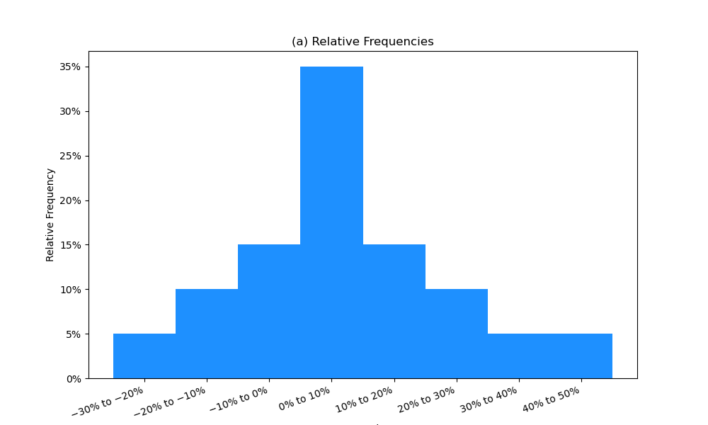
The relative frequency is another useful way to present data. The relative frequency is calculated by dividing the absolute frequency of each return interval by the total number of observations. Simply stated, relative frequency is the percentage of total observations falling within each interval. Continuing with our example, the relative frequencies are presented in the following figure.
Figure: Absolute and Relative Frequencies of Intelco Returns
| Intervals | Absolute Frequency | Relative Frequency |
|---|---|---|
| −30% ≤ Rt < −20% | 1 | 1/20 = 0.05, or 5% |
| −20% ≤ Rt < −10% | 2 | 2/20 = 0.10, or 10% |
| −10% ≤ Rt < 0% | 3 | 3/20 = 0.15, or 15% |
| 0% ≤ Rt < 10% | 7 | 7/20 = 0.35, or 35% |
| 10% ≤ Rt < 20% | 3 | 3/20 = 0.15, or 15% |
| 20% ≤ Rt < 30% | 2 | 2/20 = 0.10, or 10% |
| 30% ≤ Rt < 40% | 1 | 1/20 = 0.05, or 5% |
| 40% ≤ Rt < 50% | 1 | 1/20 = 0.05, or 5% |
| Total | 20 | 100% |
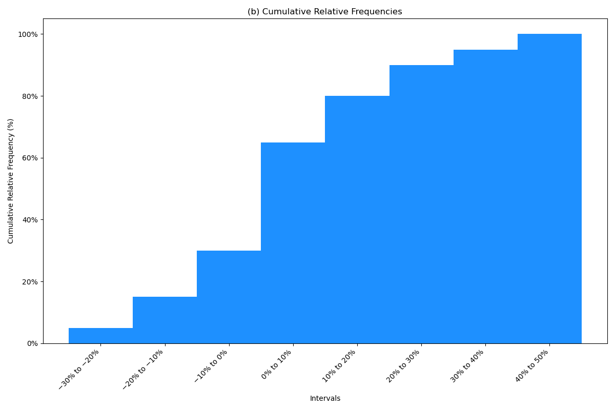
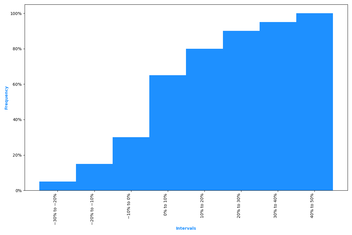
It is also possible to compute the cumulative absolute frequency and cumulative relative frequency by summing the absolute or relative frequencies starting at the lowest interval and progressing through the highest. The relative and cumulative relative frequencies for the Intelco stock returns example are presented in the following figure.
The cumulative absolute frequency or cumulative relative frequency for any given interval is the sum of the absolute or relative frequencies up to and including the given interval. For example, the cumulative absolute frequency for is and the cumulative relative frequency over this range is .
Figure: Relative and Cumulative Frequencies of Intelco Returns
D: Describe the properties of a data set presented as a histogram or a frequency polygon.
A histogram is the graphical presentation of the absolute frequency distribution. A histogram is simply a bar chart of continuous data that has been classified into a frequency distribution. The attractive feature of a histogram is that it allows us to quickly see where most of the observations are concentrated.
To construct a histogram, the intervals are scaled on the horizontal axis and the absolute frequencies are scaled on the vertical axis. The histogram for the Intelco returns data in Table B from the previous example is provided in Figure 3.
Figure 3: Histogram of Intelco Stock Return Data
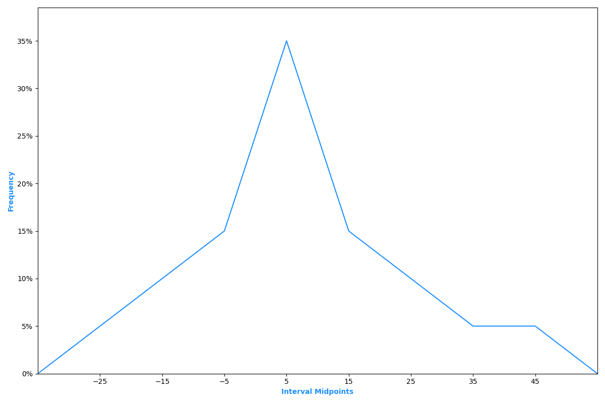
To construct a frequency polygon, the midpoint of each interval is plotted on the horizontal axis, and the absolute frequency for that interval is plotted on the vertical axis. Each point is then connected with a straight line. The frequency polygon for the returns data used in our example is illustrated in Figure 4.
Figure 4: Frequency Polygon of Intelco Stock Return Data
📝 QUIZ
- In the card game of poker, winning hands are determined by rank (high card, pair, two pair, etc.). The scale of poker hand rankings is:
- A. a nominal scale.
- B. an ordinal scale.
- C. an interval scale.
- The intervals in a frequency distribution should always have which of the following characteristics? The intervals should always:
- A. be truncated.
- B. be open ended.
- C. be nonoverlapping.
Use the following frequency distribution for Questions 3 through 5.
| Return, R | Frequency |
|---|---|
| –10% up to 0% | 3 |
| 0% up to 10% | 7 |
| 10% up to 20% | 3 |
| 20% up to 30% | 2 |
| 30% up to 40% | 1 |
- The number of intervals in this frequency table is:
- A. 1.
- B. 5.
- C. 16.
- The sample size is:
- A. 1.
- B. 5.
- C. 16
- The relative frequency of the second interval is:
- A. 10.0%.
- B. 16.0%.
- C. 43.8%.
- The vertical axis of a histogram shows:
- A. the frequency with which observations occur.
- B. the range of observations within each interval.
- C. the intervals into which the observations are arranged.
2. MEANS AND VARIANCE
E: Calculate and interpret measures of central tendency, including the population mean, sample mean, arithmetic mean, weighted average or mean, geometric mean, harmonic mean, median, and mode.
Measures of central tendency identify the center, or average, of a data set. This central point can then be used to represent the typical, or expected, value in the data set.
To compute the population mean, all the observed values in the population are summed () and divided by the number of observations in the population, N. Note that the population mean is unique in that a given population only has one mean. The population mean is expressed as:
The sample mean is the sum of all the values in a sample of a population, , divided by the number of observations in the sample, n. It is used to make inferences about the population mean. The sample mean is expressed as:
Note the use of , the sample size, versus , the population size.
You have calculated the stock returns for AXZ Corporation over the last five years as 25%, 34%, 19%, 54%, and 17%. Given this information, estimate the mean of the distribution of returns.
Answer:
The sample mean can be used as an estimate of the mean of the distribution:
The population mean and sample mean are both examples of arithmetic means. The arithmetic mean is the sum of the observation values divided by the number of observations. It is the most widely used measure of central tendency and has the following properties:
- All interval and ratio data sets have an arithmetic mean.
- All data values are considered and included in the arithmetic mean computation.
- A data set has only one arithmetic mean (i.e., the arithmetic mean is unique).
- The sum of the deviations of each observation in the data set from the mean is always zero.
The arithmetic mean is the only measure of central tendency for which the sum of the deviations from the mean is zero. Mathematically, this property can be expressed as follows:
Unusually large or small values can have a disproportionate effect on the computed value for the arithmetic mean. The mean of 1, 2, 3, and 50 is 14 and is not a good indication of what the individual data values really are. On the positive side, the arithmetic mean uses all the information available about the observations. The arithmetic mean of a sample from a population is the best estimate of both the true mean of the sample and the value of the next observation.
The computation of a weighted mean recognizes that different observations may have a disproportionate influence on the mean. The weighted mean of a set of numbers is computed with the following equation:
where:
- = observed values
- = corresponding weights associated with each of the observations such that
A portfolio consists of 50% common stocks, 40% bonds, and 10% cash. If the return on common stocks is 12%, the return on bonds is 7%, and the return on cash is 3%, what is the portfolio return?
Answer:
The example illustrates an extremely important investments concept: the return for a portfolio is the weighted average of the returns of the individual assets in the portfolio. Asset weights are market weights, the market value of each asset relative to the market value of the entire portfolio.
The median is the midpoint of a data set when the data is arranged in ascending or descending order. Half the observations lie above the median and half are below. To determine the median, arrange the data from the highest to the lowest value, or lowest to highest value, and find the middle observation.
The median is important because the arithmetic mean can be affected by extremely large or small values (outliers). When this occurs, the median is a better measure of central tendency than the mean because it is not affected by extreme values that may actually be the result of errors in the data.
What is the median return for five portfolio managers with 10-year annualized total returns record of: 30%, 15%, 25%, 21%, and 23%?
Answer:
First, arrange the returns in descending order.
30%, 25%, 23%, 21%, 15%
Then, select the observation that has an equal number of observations above and below it—the one in the middle. For the given data set, the third observation, 23%, is the median value.
Suppose we add a sixth manager to the previous example with a return of 28%. What is the median return?
Answer:
Arranging the returns in descending order gives us:
30%, 28%, 25%, 23%, 21%, 15%
With an even number of observations, there is no single middle value. The median value in this case is the arithmetic mean of the two middle observations, 25% and 23%. Thus, the median return for the six managers is 24.0% = 0.5(25 + 23).
Consider that while we calculated the mean of 1, 2, 3, and 50 as 14, the median is 2.5. If the data were 1, 2, 3, and 4 instead, the arithmetic mean and median would both be 2.5.
The mode is the value that occurs most frequently in a data set. A data set may have more than one mode or even no mode. When a distribution has one value that appears most frequently, it is said to be unimodal. When a set of data has two or three values that occur most frequently, it is said to be bimodal or trimodal, respectively.
What is the mode of the following data set?
Data set: [30%, 28%, 25%, 23%, 28%, 15%, 5%]
Answer:
The mode is 28% because it is the value appearing most frequently.
The geometric mean is often used when calculating investment returns over multiple periods or when measuring compound growth rates. The general formula for the geometric mean, , is as follows:
Note that this equation has a solution only if the product under the radical sign is non-negative.
When calculating the geometric mean for a returns data set, it is necessary to add 1 to each value under the radical and then subtract 1 from the result. The geometric mean return can be computed using the following equation:
where:
- = the return for period
For the last three years, the returns for Acme Corporation common stock have been -9.34%, 23.45%, and 8.92%. Compute the compound annual rate of return over the 3-year period.
Answer:
Solve this type of problem with your calculator as follows:
- On the TI, enter
1.21903[y^x]3[1/x][=] - On the HP, enter
1.21903[ENTER]3[1/x][y^x]
The geometric mean is always less than or equal to the arithmetic mean, and the difference increases as the dispersion of the observations increases. The only time the arithmetic and geometric means are equal is when there is no variability in the observations (i.e., all observations are equal).
A harmonic mean is used for certain computations, such as the average cost of shares purchased over time. The harmonic mean is calculated as
where there are values of .
An investor purchases $1,000 of mutual fund shares each month, and over the last three months the prices paid per share were $8, $9, and $10. What is the average cost per share?
Answer:
To check this result, calculate the total shares purchased as
The average price is
The previous example illustrates the interpretation of the harmonic mean in its most common application. Note that the average price paid per share ($8.93) is less than the arithmetic average of the share prices,
For values that are not all equal: harmonic mean geometric mean arithmetic mean. This mathematical fact is the basis for the claimed benefit of purchasing the same dollar amount of mutual fund shares each month or each week. Some refer to this practice as "dollar cost averaging."
F: Calculate and interpret quartiles, quintiles, deciles, and percentiles.
Quantile is the general term for a value at or below which a stated proportion of the data in a distribution lies. Examples of quantiles include:
- Quartiles—the distribution is divided into quarters.
- Quintile—the distribution is divided into fifths.
- Decile—the distribution is divided into tenths.
- Percentile—the distribution is divided into hundredths (percents).
Note that any quantile may be expressed as a percentile. For example, the third quartile partitions the distribution at a value such that three-fourths, or 75%, of the observations fall below that value. Thus, the third quartile is the 75th percentile.
The formula for the position of the observation at a given percentile, , with data points sorted in ascending order is:
Quantiles and measures of central tendency are known collectively as measures of location.
What is the third quartile for the following distribution of returns?
8%, 10%, 12%, 13%, 15%, 17%, 17%, 18%, 19%, 23%
Answer:
The third quartile is the point below which 75% of the observations lie. Recognizing that there are 10 observations in the data set, the third quartile can be identified as:
When the data is arranged in ascending order, the third quartile is one-fourth (0.25) of the way from the eighth data point (18%) to the ninth data point (19%), or 18.25%. This means that 75% of all observations lie below 18.25%.
G: Calculate and interpret 1) a range and a mean absolute deviation and 2) the variance and standard deviation of a population and of a sample.
Dispersion is defined as the variability around the central tendency. The common theme in finance and investments is the tradeoff between reward and variability, where the central tendency is the measure of the reward and dispersion is a measure of risk.
The range is a relatively simple measure of variability, but when used with other measures it provides extremely useful information. The range is the distance between the largest and the smallest value in the data set, or:
What is the range for the 5-year annualized total returns for five investment managers if the managers' individual returns were 30%, 12%, 25%, 20%, and 23%?
Answer:
The mean absolute deviation (MAD) is the average of the absolute values of the deviations of individual observations from the arithmetic mean.
The computation of the MAD uses the absolute values of each deviation from the mean because the sum of the actual deviations from the arithmetic mean is zero.
What is the MAD of the investment returns for the five managers discussed in the preceding example? How is it interpreted?
Answer:
annualized returns: [30%, 12%, 25%, 20%, 23%]
This result can be interpreted to mean that, on average, an individual return will deviate ±4.8% from the mean return of 22%.
The population variance is defined as the average of the squared deviations from the mean. The population variance () uses the values for all members of a population and is calculated using the following formula:
Assume the 5-year annualized total returns for the five investment managers used in the earlier example represent all of the managers at a small investment firm. What is the population variance of returns?
Answer:
Interpreting this result, we can say that the average variation from the mean return is 35.60% squared. Had we done the calculation using decimals instead of whole percents, the variance would be 0.00356. What is a percent squared? Yes, this is nonsense, but let's see what we can do so that it makes more sense.
As you have just seen, a major problem with using the variance is the difficulty of interpreting it. The computed variance, unlike the mean, is in terms of squared units of measurement. How does one interpret squared percents, squared dollars, or squared yen? This problem is mitigated through the use of the standard deviation. The population standard deviation, , is the square root of the population variance and is calculated as follows:
Using the data from the preceding examples, compute the population standard deviation.
Answer:
Calculated with decimals instead of whole percents, we would get:
Since the population standard deviation and population mean are both expressed in the same units (percent), these values are easy to relate. The outcome of this example indicates that the mean return is 22% and the standard deviation about the mean is 5.97%. Note that this is greater than the MAD of 4.8%, a result () that holds in general.
The sample variance, , is the measure of dispersion that applies when we are evaluating a sample of observations from a population. The sample variance is calculated using the following formula:
In our example for population variance, we defined the population as the returns generated by the five managers at a firm over a specific five-year period. We calculated the standard deviation of those managers’ returns for the specific five-year period. If there were 10 managers at the firm, the five returns we used would be a sample of manager returns for that firm.
In practice, we seldom have historical returns data that comprise an entire population. Consider the returns for the S&P 500 index over the last 50 years. To estimate the standard deviation of returns on the index, we would calculate the sample standard deviation, because 50 years of returns are a sample of all the possible returns outcomes for the index. The returns would be a population if we were asked to calculate the (population) standard deviation of S&P 500 returns over the specific 50-year period, rather than to estimate the standard deviation of S&P 500 returns in general.
The most noteworthy difference from the formula for population variance is that the denominator for is , one less than the sample size , where uses the entire population size . Another difference is the use of the sample mean, , instead of the population mean, . Based on the mathematical theory behind statistical procedures, the use of the entire number of sample observations, , instead of as the divisor in the computation of , will systematically underestimate the population parameter, , particularly for small sample sizes. This systematic underestimation causes the sample variance to be what is referred to as a biased estimator of the population variance. Using instead of in the denominator, however, improves the statistical properties of as an estimator of . Thus, , as expressed in the previous equation, is considered to be an unbiased estimator of .
Assume that the 5-year annualized total returns for the five investment managers used in the preceding examples represent only a sample of the managers at a large investment firm. What is the sample variance of these returns?
Answer:
Thus, the sample variance of 44.5() can be interpreted to be an unbiased estimator of the population variance. Note that 44.5 "percent squared" is 0.00445 and you will get this value if you put the percent returns in decimal form [e.g., , etc.].
As with the population standard deviation, the sample standard deviation can be calculated by taking the square root of the sample variance. The sample standard deviation, ( s ), is defined as:
Compute the sample standard deviation based on the result of the preceding example.
Answer:
Since the sample variance for the preceding example was computed to be 44.5(%(^2)), the sample standard deviation is:
The results shown here mean that the sample standard deviation, , can be interpreted as an unbiased estimator of the population standard deviation, .
📝 QUIZ
Use the following data to answer Questions 1 through 9.
XYZ Corp. Annual Stock Returns
| 2013 | 2014 | 2015 | 2016 | 2017 | 2018 |
|---|---|---|---|---|---|
| 22% | 5% | –7% | 11% | 2% | 11% |
- What is the arithmetic mean return for XYZ stock?
- A. 7.3%
- B. 8.0%
- C. 11.0%
- What is the median return for XYZ stock?
- A. 7.3%
- B. 8.0%
- C. 11.0%
- What is the mode of the returns for XYZ stock?
- A. 7.3%
- B. 8.0%
- C. 11.0%
- What is the range for XYZ stock returns?
- A. 11.0%
- B. 22.0%
- C. 29.0%
- What is the mean absolute deviation for XYZ stock returns?
- A. 5.20%
- B. 7.33%
- C. 29.0%
- Assuming that the distribution of XYZ stock returns is a population, what is the population variance?
- A. 6.8%²
- B. 7.7%²
- C. 80.2%²
- Assuming that the distribution of XYZ stock returns is a population, what is the population standard deviation?
- A. 5.02%
- B. 8.96%
- C. 46.22%
- Assuming that the distribution of XYZ stock returns is a sample, the sample variance is closest to:
- A. 5.0%²
- B. 72.4%²
- C. 96.3%²
- Assuming that the distribution of XYZ stock returns is a sample, what is the sample standard deviation?
- A. 9.8%
- B. 72.4%
- C. 96.3%
Use the following data to answer Questions 10 and 11.
The annual returns for FJW’s common stock over the years 2013, 2014, 2015, and 2016 were 15%, 19%, −8%, and 14%.
- What is the arithmetic mean return for FJW’s common stock?
- A. 10.00%.
- B. 14.00%.
- C. 15.25%.
- What is the geometric mean return for FJW’s common stock?
- A. 9.45%.
- B. 14.21%.
- C. It cannot be determined because one of the returns is negative.
- The harmonic mean of 3, 4, and 5 is:
- A. 3.74.
- B. 3.83.
- C. 4.12.
- Given the following observations:
The 65th percentile is closest to:
- A. 5.85.
- B. 6.55.
- C. 8.70.
H: Calculate and interpret the proportion of observations falling within a specified number of standard deviations of the mean using Chebyshev’s inequality.
Chebyshev’s inequality states that for any set of observations, whether sample or population data and regardless of the shape of the distribution, the percentage of the observations that lie within standard deviations of the mean is at least for all .
What is the minimum percentage of any distribution that will lie within standard deviations of the mean?
Answer:
Applying Chebyshev’s inequality, we have:
or 75%
According to Chebyshev’s inequality, the following relationships hold for any distribution. At least:
- 36% of observations lie within ±1.25 standard deviations of the mean.
- 56% of observations lie within ±1.50 standard deviations of the mean.
- 75% of observations lie within ±2 standard deviations of the mean.
- 89% of observations lie within ±3 standard deviations of the mean.
- 94% of observations lie within ±4 standard deviations of the mean.
The importance of Chebyshev’s inequality is that it applies to any distribution. If we actually know the underlying distribution is normal, for example, we can be even more precise about the percentage of observations that will fall within 2 or 3 standard deviations of the mean.
I: Calculate and interpret the coefficient of variation.
A direct comparison between two or more measures of dispersion may be difficult. For instance, suppose you are comparing the annual returns distribution for retail stocks with a mean of 8% and an annual returns distribution for a real estate portfolio with a mean of 16%. A direct comparison between the dispersion of the two distributions is not meaningful because of the relatively large difference in their means. To make a meaningful comparison, a relative measure of dispersion must be used. Relative dispersion is the amount of variability in a distribution relative to a reference point or benchmark. Relative dispersion is commonly measured with the coefficient of variation (), which is computed as:
measures the amount of dispersion in a distribution relative to the distribution’s mean. It is useful because it enables us to make a direct comparison of dispersion across different sets of data. In an investments setting, the CV is used to measure the risk (variability) per unit of expected return (mean).
You have just been presented with a report that indicates that the mean monthly return on T-bills is 0.25% with a standard deviation of 0.36%, and the mean monthly return for the S&P 500 is 1.09% with a standard deviation of 7.30%. Your unit manager has asked you to compute the CV for these two investments and to interpret your results.
Answer:
These results indicate that there is less dispersion (risk) per unit of monthly return for T-bills than there is for the S&P 500 (1.44 versus 6.70).
To remember the formula for CV, remember that the coefficient of variation is a measure of variation, so standard deviation goes in the numerator. CV is variation per unit of return.
J: Explain skewness and the meaning of a positively or negatively skewed return distribution.
A distribution is symmetrical if it is shaped identically on both sides of its mean. Distributional symmetry implies that intervals of losses and gains will exhibit the same frequency. For example, a symmetrical distribution with a mean return of zero will have losses in the –6% to –4% interval as frequently as it will have gains in the +4% to +6% interval. The extent to which a returns distribution is symmetrical is important because the degree of symmetry tells analysts if deviations from the mean are more likely to be positive or negative.
Skewness, or skew, refers to the extent to which a distribution is not symmetrical. Nonsymmetrical distributions may be either positively or negatively skewed and result from the occurrence of outliers in the data set. Outliers are observations with extraordinarily large values, either positive or negative.
-
A positively skewed distribution is characterized by many outliers in the upper region, or right tail. A positively skewed distribution is said to be skewed right because of its relatively long upper (right) tail.
-
A negatively skewed distribution has a disproportionately large amount of outliers that fall within its lower (left) tail. A negatively skewed distribution is said to be skewed left because of its long lower tail.
K: Describe the relative locations of the mean, median, and mode for a unimodal, nonsymmetrical distribution.
Skewness affects the location of the mean, median, and mode of a distribution.
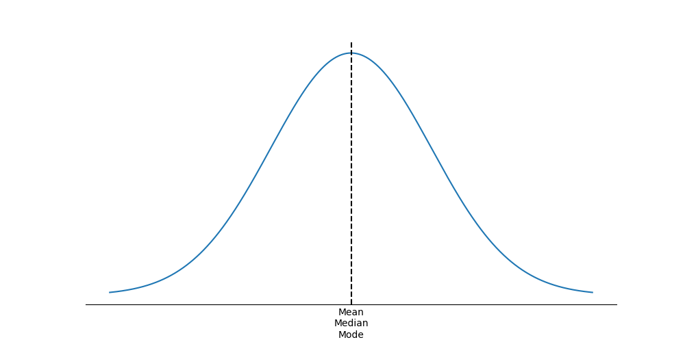
- For a symmetrical distribution, the mean, median, and mode are equal.
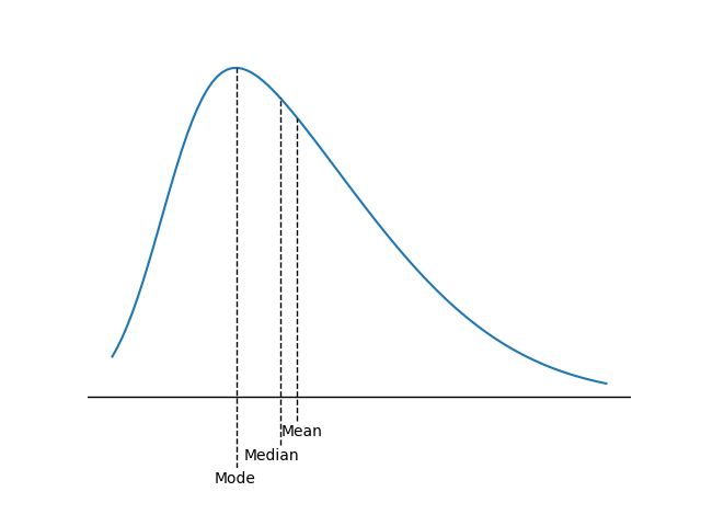
- For a positively skewed, unimodal distribution, the mode is less than the median, which is less than the mean. The mean is affected by outliers; in a positively skewed distribution, there are large, positive outliers which will tend to “pull” the mean upward, or more positive.
- An example of a positively skewed distribution is that of housing prices. Suppose that you live in a neighborhood with 100 homes; 99 of them sell for $100,000, and one sells for $1,000,000. The median and the mode will be $100,000, but the mean will be $109,000. Hence, the mean has been “pulled” upward (to the right) by the existence of one home (outlier) in the neighborhood.
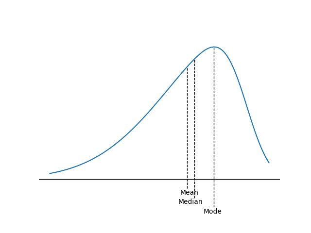
- For a negatively skewed, unimodal distribution, the mean is less than the median, which is less than the mode. In this case, there are large, negative outliers that tend to “pull” the mean downward (to the left).
The key to remembering how measures of central tendency are affected by skewed data is to recognize that skew affects the mean more than the median and mode, and the mean is “pulled” in the direction of the skew. The relative location of the mean, median, and mode for different distribution shapes is shown in the following figures. Note the median is between the other two measures for positively or negatively skewed distributions.
Figures: Effect of Skewness on Mean, Median, and Mode
Symmetrical ()
Positive (right) skew ()
Negative (left) skew ()
L: Explain measures of sample skewness and kurtosis.
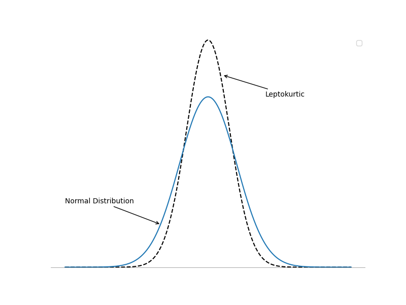
Kurtosis is a measure of the degree to which a distribution is more or less “peaked” than a normal distribution. Leptokurtic describes a distribution that is more peaked than a normal distribution, whereas platykurtic refers to a distribution that is less peaked, or flatter than a normal distribution. A distribution is mesokurtic if it has the same kurtosis as a normal distribution.
As indicated in the following figure, a leptokurtic return distribution will have more returns clustered around the mean and more returns with large deviations from the mean (fatter tails). Relative to a normal distribution, a leptokurtic distribution will have a greater percentage of small deviations from the mean and a greater percentage of extremely large deviations from the mean. This means that there is a relatively greater probability of an observed value being either close to the mean or far from the mean. With regard to an investment returns distribution, a greater likelihood of a large deviation from the mean return is often perceived as an increase in risk.
Figure: Kurtosis
A distribution is said to exhibit excess kurtosis if it has either more or less kurtosis than the normal distribution. The computed kurtosis for all normal distributions is three. Statisticians, however, sometimes report excess kurtosis, which is defined as kurtosis minus three. Thus, a normal distribution has excess kurtosis equal to zero, a leptokurtic distribution has excess kurtosis greater than zero, and platykurtic distributions will have excess kurtosis less than zero.
Kurtosis is critical in a risk management setting. Most research about the distribution of securities returns has shown that returns are not normally distributed. Actual securities returns tend to exhibit both skewness and kurtosis. Skewness and kurtosis are critical concepts for risk management because when securities returns are modeled using an assumed normal distribution, the predictions from the models will not take into account the potential for extremely large, negative outcomes. In fact, most risk managers put very little emphasis on the mean and standard deviation of a distribution and focus more on the distribution of returns in the tails of the distribution—that is where the risk is. In general, greater positive kurtosis and more negative skew in returns distributions indicates increased risk.
Measures of Sample Skew and Kurtosis
Sample skewness is equal to the sum of the cubed deviations from the mean divided by the cubed standard deviation and by the number of observations. Sample skewness for large samples is computed as:
where:
- = sample standard deviation
Note that the denominator is always positive, but that the numerator can be positive or negative, depending on whether observations above the mean or observations below the mean tend to be further from the mean on average. When a distribution is right skewed, sample skewness is positive because the deviations above the mean are larger on average. A left-skewed distribution has a negative sample skewness.
Dividing by standard deviation cubed standardizes the statistic and allows interpretation of the skewness measure. If relative skewness is equal to zero, the data is not skewed. Positive levels of relative skewness imply a positively skewed distribution, whereas negative values of relative skewness imply a negatively skewed distribution. Values of sample skewness in excess of in absolute value are considered significant.
Sample kurtosis is measured using deviations raised to the fourth power.
where:
- = sample standard deviation
To interpret kurtosis, note that it is measured relative to the kurtosis of a normal distribution, which is . Positive values of excess kurtosis indicate a distribution that is leptokurtic (more peaked, fat tails), whereas negative values indicate a platykurtic distribution (less peaked, thin tails). Excess kurtosis values that exceed 1.0 in absolute value are considered large. We can calculate kurtosis relative to that of a normal distribution as:
M: Compare the use of arithmetic and geometric means when analyzing investment returns.
Since past annual returns are compounded each period, the geometric mean of past annual returns is the appropriate measure of past performance. It gives us the average annual compound return. With annual returns of 10%, 15%, -4%, 9%, and 5% over five years, the geometric mean return of tells us the single rate that, if compounded over the five periods, would lead to the same increase in wealth as the individual annual rates of return.
The arithmetic mean of is, however, the statistically best estimator of the next year's returns given only the five years of return outcomes. To estimate multi-year returns (e.g. expected annual return over the next three years), the geometric mean of 6.81% is the appropriate measure.
Consider also a forward-looking model where returns will be either +100% or -50% each year for two years. Note that when returns are +100% in Year 1 and -50% in Year 2, the annual geometric mean return is and the arithmetic mean annual return is .
Consider the following tree model for two years where the outcomes of +100% and -50% are equally likely and beginning wealth is $1,000:
                 $4,000 (Prob = 25%)
               /
        $2,000
       /       \
$1,000           $1,000 (Prob = 50%)
       \       /
         $500
               \
                  $250  (Prob = 25%)
Each of the four possible ending wealth values has a 25% probability, so the expected ending wealth is simply
This is consistent with earning a compound annual rate of return equal to the arithmetic mean of 25%, , but not with earning the geometric mean return of 0%. For each single year, the expected rate of return is simply the average of and since those outcomes are equally likely.
📝 QUIZ
- For a skewed distribution, what is the minimum percentage of the observations that will lie between ±2.5 standard deviations of the mean based on Chebyshev’s Inequality?
- A. 56%.
- B. 75%.
- C. 84%.
- A distribution of returns that has a greater percentage of small deviations from the mean and a greater percentage of extremely large deviations from the mean compared to a normal distribution:
- A. is positively skewed.
- B. has positive excess kurtosis.
- C. has negative excess kurtosis.
- Which of the following is most accurate regarding a distribution of returns that has a mean greater than its median?
- A. It is positively skewed.
- B. It is a symmetric distribution.
- C. It has positive excess kurtosis.
- A normal distribution has kurtosis of:
- A. zero.
- B. one.
- C. three.
- The most appropriate measure of central tendency for forecasting an investment return in a single future period is:
- A. the harmonic mean.
- B. the arithmetic mean.
- C. the geometric mean.