Sampling and Estimation

This topic review covers random samples and inferences about population means from sample data. It is essential that you know the central limit theorem, for it allows us to use sampling statistics to construct confidence intervals for point estimates of population means. Make sure you can calculate confidence intervals for population means given sample parameter estimates and a level of significance, and know when it is appropriate to use the $z$-statistic versus the $t$-statistic. You should also understand the basic procedures for creating random samples, and recognize the warning signs of various sampling biases from nonrandom samples.

1: CENTRAL LIMIT THEORM AND STANDARD ERROR

In many real-world statistics applications, it is impractical (or impossible) to study an entire population. When this is the case, a subgroup of the population, called a sample, can be evaluated. Based upon this sample, the parameters of the underlying population can be estimated.

For example, rather than attempting to measure the performance of the U.S. stock market by observing the performance of all 10,000 or so stocks trading in the United States at any one time, the performance of the subgroup of 500 stocks in the S&P 500 can be measured. The results of the statistical analysis of this sample can then be used to draw conclusions about the entire population of U.S. stocks.

A: Define simple random sampling and a sampling distribution.

B: Explain sampling error.

Simple random sampling is a method of selecting a sample in such a way that each item or person in the population being studied has the same likelihood of being included in the sample. As an example of simple random sampling, assume that you want to draw a sample of five items out of a group of 50 items. This can be accomplished by numbering each of the 50 items, placing them in a hat, and shaking the hat. Next, one number can be drawn randomly from the hat. Repeating this process (experiment) four more times results in a set of five numbers. The five drawn numbers (items) comprise a simple random sample from the population. In applications like this one, a random-number table or a computer random number generator is often used to create the sample. Another way to form an approximately random sample is systematic sampling, selecting every nth member from a population. Sampling error is the difference between a sample statistic (the mean, variance, or standard deviation of the sample) and its corresponding population parameter (the true mean, variance, or standard deviation of the population). For example, the sampling error for the mean is as follows:

$$\text{sampling error of the mean} = \text{sample mean} - \text{population mean} = \bar{x} - \mu$$

A Sampling Distribution

It is important to recognize that the sample statistic itself is a random variable and, therefore, has a probability distribution. The sampling distribution of the sample statistic is a probability distribution of all possible sample statistics computed from a set of equal-size samples that were randomly drawn from the same population. Think of it as the probability distribution of a statistic from many samples.

For example, suppose a random sample of 100 bonds is selected from a population of a major municipal bond index consisting of 1,000 bonds, and then the mean return of the 100-bond sample is calculated. Repeating this process many times will result in many different estimates of the population mean return (i.e., one for each sample). The distribution of these estimates of the mean is the sampling distribution of the mean.

It is important to note that this sampling distribution is distinct from the distribution of the actual prices of the 1,000 bonds in the underlying population and will have different parameters.

C: Distinguish between simple random and stratified random sampling.

Stratified random sampling uses a classification system to separate the population into smaller groups based on one or more distinguishing characteristics. From each subgroup, or stratum, a random sample is taken and the results are pooled. The size of the samples from each stratum is based on the size of the stratum relative to the population.

Stratified sampling is often used in bond indexing because of the difficulty and cost of completely replicating the entire population of bonds. In this case, bonds in a population are categorized (stratified) according to major bond risk factors such as duration, maturity, coupon rate, and the like. Then, samples are drawn from each separate category and combined to form a final sample.

To see how this works, suppose you want to construct a bond portfolio that is indexed to the major municipal bond index using a stratified random sampling approach. First, the entire population of 1,000 municipal bonds in the index can be classified on the basis of maturity and coupon rate. Then, cells (stratum) can be created for different maturity/coupon combinations, and random samples can be drawn from each of the maturity/coupon cells. To sample from a cell containing 50 bonds with 2- to 4-year maturities and coupon rates less than 5%, we would select five bonds. The number of bonds drawn from a given cell corresponds to the cell’s weight relative to the population (index), or (50 / 1000) x (100) = 5 bonds. This process is repeated for all of the maturity/coupon cells, and the individual samples are combined to form the portfolio.

By using stratified sampling, we guarantee that we sample five bonds from this cell. If we had used simple random sampling, there would be no guarantee that we would sample any of the bonds in the cell. Or, we may have selected more than five bonds from this cell.

D: Distinguish between time-series and cross-sectional data.

Time-series data consist of observations taken over a period of time at specific and equally spaced time intervals. The set of monthly returns on Microsoft stock from January 1994 to January 2004 is an example of a time-series data sample.

Cross-sectional data are a sample of observations taken at a single point in time. The sample of reported earnings per share of all Nasdaq companies as of December 31, 2004, is an example of a cross-sectional data sample.

Time-series and cross-sectional data can be pooled in the same data set. Longitudinal data are observations over time of multiple characteristics of the same entity, such as unemployment, inflation, and GDP growth rates for a country over 10 years. Panel data contain observations over time of the same characteristic for multiple entities, such as debt/equity ratios for 20 companies over the most recent 24 quarters. Panel and longitudinal data are typically presented in table or spreadsheet form.

E: Explain the central limit theorem and its importance.

The central limit theorem states that for simple random samples of size n from a population with a mean $μ$ and a finite variance $\sigma^2$, the sampling distribution of the sample mean $\bar{x}$ approaches a normal probability distribution with mean μ and a variance equal to $\frac{\sigma^2}{n}$ as the sample size becomes large.

The central limit theorem is extremely useful because the normal distribution is relatively easy to apply to hypothesis testing and to the construction of confidence intervals. Specific inferences about the population mean can be made from the sample mean, regardless of the population’s distribution, as long as the sample size is “sufficiently large,” which usually means n ≥ 30.

Important properties of the central limit theorem include the following:

• If the sample size n is sufficiently large (n ≥ 30), the sampling distribution of the sample means will be approximately normal. Remember what’s going on here, random samples of size n are repeatedly being taken from an overall larger population. Each of these random samples has its own mean, which is itself a random variable, and this set of sample means has a distribution that is approximately normal.
• The mean of the population, μ, and the mean of the distribution of all possible sample means are equal.
• The variance of the distribution of sample means is $\frac{\sigma^2}{n}$, the population variance divided by the sample size.

F: Calculate and interpret the standard error of the sample mean.

The standard error of the sample mean is the standard deviation of the distribution of the sample means.

When the standard deviation of the population, $\sigma$, is known, the standard error of the sample mean is calculated as:

$$\sigma_{\bar{x}} = \frac{\sigma}{\sqrt{n}}$$

where:

• $\sigma_{\bar{x}}$ = standard error of the sample mean
• $\sigma$ = standard deviation of the population
• $n$ = size of the sample

EXAMPLE: Standard error of sample mean (known population variance)

The mean hourly wage for Iowa farm workers is $13.50 with a population standard deviation of $2.90. Calculate and interpret the standard error of the sample mean for a sample size of 30.

Answer:

Because the population standard deviation, $\sigma$, is known, the standard error of the sample mean is expressed as:

$$\sigma_{\bar{x}} = \frac{\sigma}{\sqrt{n}} = \frac{2.90}{\sqrt{30}} = \$0.53$$

This means that if we were to take many samples of size 30 from the Iowa farm worker population and prepare a sampling distribution of the sample means, we would get a distribution with an expected mean of $13.50 and standard error (standard deviation of the sample means) of $0.53.

Practically speaking, the population’s standard deviation is almost never known. Instead, the standard error of the sample mean must be estimated by dividing the standard deviation of the sample by $\sqrt{n}$:

$$s_{\bar{x}} = \frac{s}{\sqrt{n}}$$

EXAMPLE: Standard error of sample mean (unknown population variance)

Suppose a sample contains the past 30 monthly returns for McCreary, Inc. The mean return is 2% and the sample standard deviation is 20%. Calculate and interpret the standard error of the sample mean.

Answer:

Since $\sigma$ is unknown, the standard error of the sample mean is:

$$s_{\bar{x}} = \frac{s}{\sqrt{n}} = \frac{20\%}{\sqrt{30}} = 3.6\%$$

This implies that if we took all possible samples of size 30 from McCreary’s monthly returns and prepared a sampling distribution of the sample means, the mean would be 2% with a standard error of 3.6%.

EXAMPLE: Standard error of sample mean (unknown population variance)

Continuing with our example, suppose that instead of a sample size of 30, we take a sample of the past 200 monthly returns for McCreary, Inc. In order to highlight the effect of sample size on the sample standard error, let’s assume that the mean return and standard deviation of this larger sample remain at 2% and 20%, respectively. Now, calculate the standard error of the sample mean for the 200-return sample.

Answer:

The standard error of the sample mean is computed as:

$$s_{\bar{x}} = \frac{s}{\sqrt{n}} = \frac{20\%}{\sqrt{200}} = 1.4\%$$

The result of the preceding two examples illustrates an important property of sampling distributions. Notice that the value of the standard error of the sample mean decreased from 3.6% to 1.4% as the sample size increased from 30 to 200. This is because as the sample size increases, the sample mean gets closer, on average, to the true mean of the population. In other words, the distribution of the sample means about the population mean gets smaller and smaller, so the standard error of the sample mean decreases.

PROFESSOR'S NOTE

I get a lot of questions about when to use $\sigma$ and $\sigma / \sqrt{n}$. Just remember that the standard deviation of the means of multiple samples is less than the standard deviation of single observations. If the standard deviation of monthly stock returns is 2%, the standard error (deviation) of the average monthly return over the next six months is $2\% / \sqrt{6} = 0.82\%$. The average of several observations of a random variable will be less widely dispersed (have lower standard deviation) around the expected value than will a single observation of the random variable.

G: Identify and describe desirable properties of an estimator.

Regardless of whether we are concerned with point estimates or confidence intervals, there are certain statistical properties that make some estimators more desirable than others. These desirable properties of an estimator are unbiasedness, efficiency, and consistency.

• An unbiased estimator is one for which the expected value of the estimator is equal to the parameter you are trying to estimate. For example, because the expected value of the sample mean is equal to the population mean $\mathbb{E}(\bar{x}) = \mu$, the sample mean is an unbiased estimator of the population mean.
• An unbiased estimator is also efficient if the variance of its sampling distribution is smaller than all the other unbiased estimators of the parameter you are trying to estimate. The sample mean, for example, is an unbiased and efficient estimator of the population mean.
• A consistent estimator is one for which the accuracy of the parameter estimate increases as the sample size increases. As the sample size increases, the standard error of the sample mean falls, and the sampling distribution bunches more closely around the population mean. In fact, as the sample size approaches infinity, the standard error approaches zero.

📝 QUIZ

1. A simple random sample is a sample drawn in such a way that each member of the population has:

• A. some chance of being selected in the sample.
• B. an equal chance of being included in the sample.
• C. a 1% chance of being included in the sample.

2. The sampling distribution of a statistic is the probability distribution made up of all possible:

• A. observations from the underlying population.
• B. sample statistics computed from samples of varying sizes drawn from the same population.
• C. sample statistics computed from samples of the same size drawn from the same population.

3. Sampling error is defined as:

• A. an error that occurs when a sample of less than 30 elements is drawn.
• B. an error that occurs during collection, recording, and tabulation of data.
• C. the difference between the value of a sample statistic and the value of the corresponding population parameter.

4. The mean age of all CFA candidates is 28 years. The mean age of a random sample of 100 candidates is found to be 26.5 years. The difference of 1.5 years is called:

• A. the random error.
• B. the sampling error.
• C. the population error.

5. The sample of debt/equity ratios of 25 publicly traded U.S. banks as of fiscal year-end 2003 is an example of:

• A. a point estimate.
• B. cross-sectional data.
• C. a stratified random sample.

6. To apply the central limit theorem to the sampling distribution of the sample mean, the sample is usually considered to be large if $n$ is greater than:

• A. 20.
• B. 25.
• C. 30.

7. If $n$ is large and the population standard deviation is unknown, the standard error of the sampling distribution of the sample mean is equal to:

• A. the sample standard deviation divided by the sample size.
• B. the population standard deviation multiplied by the sample size.
• C. the sample standard deviation divided by the square root of the sample size.

8. The standard error of the sampling distribution of the sample mean for a sample size of $n$ drawn from a population with a mean of $\mu$ and a standard deviation of $\sigma$ is:

• A. sample standard deviation divided by the sample size.
• B. sample standard deviation divided by the square root of the sample size.
• C. population standard deviation divided by the square root of the sample size.

9. Assume that a population has a mean of 14 with a standard deviation of 2. If a random sample of 49 observations is drawn from this population, the standard error of the sample mean is closest to:

• A. 0.04.
• B. 0.29.
• C. 2.00.

10. The population’s mean is 30 and the mean of a sample of size 100 is 28.5. The variance of the sample is 25. The standard error of the sample mean is closest to:

• A. 0.05.
• B. 0.25.
• C. 0.50.

11. Which of the following is least likely a desirable property of an estimator?

• A. Reliability.
• B. Efficiency.
• C. Consistency.

2: CONFIDENCE INTERVALS AND t-DISTRIBUTION

H: Distinguish between a point estimate and a confidence interval estimate of a population parameter.

Point estimates are single (sample) values used to estimate population parameters. The formula used to compute the point estimate is called the estimator. For example, the sample mean, $\bar{x}$, is an estimator of the population mean $\mu$ and is computed using the familiar formula:

$$\bar{x} = \frac{\sum x}{n}$$

The value generated with this calculation for a given sample is called the point estimate of the mean.

A confidence interval is a range of values in which the population parameter is expected to lie. The construction of confidence intervals is described later in this topic review.

I: Describe properties of Student’s t-distribution and calculate and interpret its degrees of freedom.

Student’s t-distribution, or simply the t-distribution, is a bell-shaped probability distribution that is symmetrical about its mean. It is the appropriate distribution to use when constructing confidence intervals based on small samples (n < 30) from populations with unknown variance and a normal, or approximately normal, distribution. It may also be appropriate to use the t-distribution when the population variance is unknown and the sample size is large enough that the central limit theorem will assure that the sampling distribution is approximately normal.

Student’s t-distribution has the following properties:

• It is symmetrical.
• It is defined by a single parameter, the degrees of freedom ($df$), where the degrees of freedom are equal to the number of sample observations minus 1, $n – 1$, for sample means.
• It has more probability in the tails (“fatter tails”) than the normal distribution.
• As the degrees of freedom (the sample size) gets larger, the shape of the t-distribution more closely approaches a standard normal distribution.

When compared to the normal distribution, the t-distribution is flatter with more area under the tails (i.e., it has fatter tails). As the degrees of freedom for the t-distribution increase, however, its shape approaches that of the normal distribution.

The degrees of freedom for tests based on sample means are $n – 1$ because, given the mean, only $n – 1$ observations can be unique.

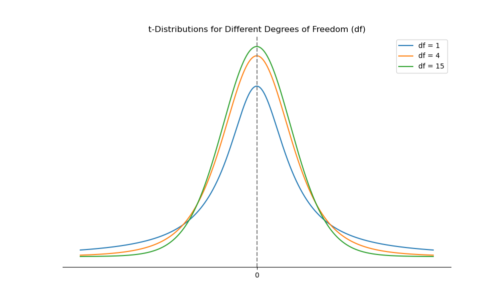
The t-distribution is a symmetrical distribution that is centered about zero. The shape of the t-distribution is dependent on the number of degrees of freedom, and degrees of freedom are based on the number of sample observations. The t-distribution is flatter and has thicker tails than the standard normal distribution. As the number of observations increases (i.e., the degrees of freedom increase), the $t$-distribution becomes more spiked and its tails become thinner. As the number of degrees of freedom increases without bound, the t-distribution converges to the standard normal distribution ($z$-distribution). The thickness of the tails relative to those of the $z$-distribution is important in hypothesis testing because thicker tails mean more observations away from the center of the distribution (more outliers). Hence, hypothesis testing using the $t$-distribution makes it more difficult to reject the null relative to hypothesis testing using the $z$-distribution.

The following table contains one-tailed critical values for the $t$-distribution at the 0.05 and 0.025 levels of significance with various degrees of freedom ($df$). Note that, unlike the $z$-table, the $t$-values are contained within the table, and the probabilities are located at the column headings. Also note that the level of significance of a $t$-test corresponds to the one-tailed probabilities, p, that head the columns in the t-table.

Table of Critical t-Values

One-Tailed Probabilities, p
df	p = 0.05	p = 0.025
5	2.015	2.571
10	1.812	2.228
15	1.753	2.131
20	1.725	2.086
25	1.708	2.060
30	1.697	2.042
40	1.684	2.021
50	1.676	2.009
60	1.671	2.000
70	1.667	1.994
80	1.664	1.990
90	1.662	1.987
100	1.660	1.984
120	1.658	1.980
∞	1.645	1.960

The following figure illustrates the different shapes of the $t$-distribution associated with different degrees of freedom. The tendency is for the $t$-distribution to look more and more like the normal distribution as the degrees of freedom increase. Practically speaking, the greater the degrees of freedom, the greater the percentage of observations near the center of the distribution and the lower the percentage of observations in the tails, which are thinner as degrees of freedom increase. This means that confidence intervals for a random variable that follows a $t$-distribution must be wider (narrower) when the degrees of freedom are less (more) for a given significance level.

Figure: $t$-Distributions for Different Degrees of Freedom ($\text{df}$)

J: Calculate and interpret a confidence interval for a population mean, given a normal distribution with 1) a known population variance, 2) an unknown population variance, or 3) an unknown population variance and a large sample size.

Confidence interval estimates result in a range of values within which the actual value of a parameter will lie, given the probability of $1 - \alpha$. Here, alpha, $\alpha$, is called the level of significance for the confidence interval, and the probability $1 - \alpha$ is referred to as the degree of confidence. For example, we might estimate that the population mean of random variables will range from 15 to 25 with a 95$\%$ degree of confidence, or at the 5$\%$ level of significance.

Confidence intervals are usually constructed by adding or subtracting an appropriate value from the point estimate. In general, confidence intervals take on the following form:

$$\text{point estimate} \pm (\text{reliability factor} \times \text{standard error})$$

where:

• point estimate = value of a sample statistic of the population parameter
• reliability factor = number that depends on the sampling distribution of the point estimate and the probability that the point estimate falls in the confidence interval, $1 - \alpha$
• standard error = standard error of the point estimate

If the population has a normal distribution with a known variance, a confidence interval for the population mean can be calculated as:

$$\bar{x} \pm z_{\alpha/2} \frac{\sigma}{\sqrt{n}}$$

where:

• $\bar{x}$ = point estimate of the population mean (sample mean).
• $z_{\alpha/2}$ = reliability factor, a standard normal random variable for which the probability in the right-hand tail of the distribution is $\alpha/2$. In other words, this is the z-score that leaves $\alpha/2$ of probability in the upper tail.
• $\frac{\sigma}{\sqrt{n}}$ = the standard error of the sample mean where $\sigma$ is the known standard deviation of the population, and $n$ is the sample size.

The most commonly used standard normal distribution reliability factors are:

$$z_{\alpha/2} = 1.645 \text{ for 90\% confidence intervals (the significance level is 10\%, 5\% in each tail).}$$ $$z_{\alpha/2} = 1.960 \text{ for 95\% confidence intervals (the significance level is 5\%, 2.5\% in each tail).}$$ $$z_{\alpha/2} = 2.575 \text{ for 99\% confidence intervals (the significance level is 1\%, 0.5\% in each tail).}$$

Do these numbers look familiar? They should! In our review of common probability distributions, we found the probability under the standard normal curve between z = –1.96 and z = +1.96 to be 0.95, or 95%. Owing to symmetry, this leaves a probability of 0.025 under each tail of the curve beyond z = –1.96 or z = +1.96, for a total of 0.05, or 5%—just what we need for a significance level of 0.05, or 5%.

EXAMPLE: Confidence interval

Consider a practice exam that was administered to 36 Level I candidates. The mean score on this practice exam was 80. Assuming a population standard deviation equal to 15, construct and interpret a 99% confidence interval for the mean score on the practice exam for 36 candidates. Note that in this example the population standard deviation is known, so we don’t have to estimate it.

Answer: At a confidence level of 99%, $z_{\alpha/2} = z_{0.005} = 2.58$. So, the 99% confidence interval is calculated as follows:

$$\bar{x} \pm z_{\alpha/2} \frac{\sigma}{\sqrt{n}} = 80 \pm 2.58 \frac{15}{\sqrt{36}} = 80 \pm 6.45$$

Thus, the 99% confidence interval ranges from 73.55 to 86.45.

EXAMPLE: Confidence intervals for a population mean and for a single observation

Annual returns on energy stocks are approximately normally distributed with a mean of 9% and standard deviation of 6%. Construct a 90% confidence interval for the annual returns of a randomly selected energy stock and a 90% confidence interval for the mean of the annual returns for a sample of 12 energy stocks.

Answer: A 90% confidence interval for a single observation is 1.645 standard deviations from the sample mean.

$$9\% \pm 1.645(6\%) = -0.87\% \text{ to } 18.87\%$$

A 90% confidence interval for the population mean is 1.645 standard errors from the sample mean.

$$9\% \pm 1.645 \left( \frac{6\%}{\sqrt{12}} \right) = 6.15\% \text{ to } 11.85\%$$

Confidence intervals can be interpreted from a probabilistic perspective or a practical perspective. With regard to the outcome of the $\text{CFA}^\circledR$ practice exam example, these two perspectives can be described as follows:

• Probabilistic interpretation. After repeatedly taking samples of CFA candidates, administering the practice exam, and constructing confidence intervals for each sample’s mean, 99% of the resulting confidence intervals will, in the long run, include the population mean.
• Practical interpretation. We are 99% confident that the population mean score is between 73.55 and 86.45 for candidates from this population.

Confidence Intervals for the Population Mean: Normal With Unknown Variance

If the distribution of the population is normal with unknown variance, we can use the t-distribution to construct a confidence interval:

$$\bar{x} \pm t_{\alpha/2} \frac{s}{\sqrt{n}}$$

where:

• $\bar{x}$ = the point estimate of the population mean
• $t_{\alpha/2}$ = the reliability factor (a.k.a. t-statistic or critical t-value) corresponding to a t-distributed random variable with $n - 1$ degrees of freedom, where $n$ is the sample size. The area under the tail of the t-distribution to the right of $t_{\alpha/2}$ is $\alpha/2$
• $\frac{s}{\sqrt{n}}$ = standard error of the sample mean
• $s$ = sample standard deviation

Unlike the standard normal distribution, the reliability factors for the t-distribution depend on the sample size, so we can’t rely on a commonly used set of reliability factors. Instead, reliability factors for the t-distribution have to be looked up in a table of Student’s t-distribution, like the one at the back of this book.

Owing to the relatively fatter tails of the t-distribution, confidence intervals constructed using t-reliability factors $(t_{\alpha/2})$ will be more conservative (wider) than those constructed using z-reliability factors $(z_{\alpha/2})$.

EXAMPLE: Confidence intervals

Let's return to the McCrary, Inc. example. Recall that we took a sample of the past 30 monthly stock returns for McCrary, Inc. and determined that the mean return was 2% and the sample standard deviation was 20%. Since the population variance is unknown, the standard error of the sample was estimated to be: $s_{\bar{x}} = \frac{s}{\sqrt{n}} = \frac{20\%}{\sqrt{30}} = 3.65\%$

Now, let’s construct a 95% confidence interval for the mean monthly return.

Answer: Here, we will use the reliability factor because the population variance is unknown. Since there are 30 observations, the degrees of freedom are $n - 1 = 30 - 1 = 29$. Remember, because this is a two-tailed test, at the 95% confidence level, the probability under each tail must be $\alpha/2 = 2.5\%$, for a total of 5%. So, referencing the one-sided probabilities for Student’s t-distribution at the back of this book, we find the critical t-value (reliability factor) at $\alpha/2 = 0.025$ and $n - 1 = 29$ to be $t_{\alpha/2} = 2.045$. Thus, the 95% confidence interval for the population mean is: $2\% \pm (t_{\alpha/2} \cdot s_{\bar{x}}) = 2\% \pm 2.045 (3.65\%) = 2\% \pm 7.4\%$

Thus, the 95% confidence has a lower limit of -5.4% and an upper limit of 9.4%.

We can interpret this confidence interval by saying that we are 95% confident that the population mean monthly return for McCrary stock is between -5.4% and 9.4%.

PROFESSOR'S NOTE

You should practice looking up reliability factors (i.e., critical t-values or t-statistics) in a t-table. The first step is always to compute the degrees of freedom, which is $n - 1$. The second step is to find the appropriate level of alpha or significance. This depends on whether the test you’re concerned with is one-tailed (like our example) or two-tailed (like our example).

Confidence Interval for a Population Mean When the Population Variance Is Unknown Given a Large Sample From Any Type of Distribution

We now know that the $z$-statistic should be used to construct confidence intervals when the population distribution is normal and the variance is known, and the t-statistic should be used when the distribution is normal but the variance is unknown. But what do we do when the distribution is nonnormal?

As it turns out, the size of the sample influences whether or not we can construct the appropriate confidence interval for the sample mean.

• If the distribution is normal but the population variance is unknown, the $z$-statistic can be used as long as the sample size is large ($n \ge 30$). We can do this because the central limit theorem assures us that the distribution of the sample mean is approximately normal when the sample is large.
• If the distribution is nonnormal and the population variance is unknown, the $t$-statistic can be used as long as the sample size is large ($n \ge 30$). It is also acceptable to use the $z$-statistic, although use of the t-statistic is more conservative.

This means that if we are sampling from a nonnormal distribution (which is sometimes the case in finance), we cannot create a confidence interval if the sample size is less than 30. So, all else equal, make sure you have a sample of at least 30, and the larger, the better.

PROFESSOR'S NOTE

You should commit the criteria in the following table to memory.

Table: Criteria for Selecting the Appropriate Test Statistic

	Test Statistic	Test Statistic
When sampling from a:	Small Sample ($n < 30$)	Large Sample ($n \ge 30$)
Normal distribution with known variance	z-statistic	z-statistic
Normal distribution with unknown variance	t-statistic	t-statistic
Nonnormal distribution with known variance	not available	z-statistic
Nonnormal distribution with unknown variance	not available	t-statistic

Note: The t-statistic is theoretically acceptable here, but use of the t-statistic is more conservative.

All of the preceding analysis depends on the sample we draw from the population being random. If the sample isn't random, the central limit theorem doesn't apply, our estimates won't have the desirable properties, and we can't form unbiased confidence intervals. Surprisingly, creating a random sample is not as easy as one might believe. There are a number of potential mistakes in sampling methods that can bias the results. These biases are particularly problematic in financial research, where available historical data are plentiful, but the creation of new sample data by experimentation is restricted.

K: Describe the issues regarding selection of the appropriate sample size, data- mining bias, sample selection bias, survivorship bias, look-ahead bias, and time-period bias.

We have seen so far that a larger sample reduces the sampling error and the standard deviation of the sample statistic around its true (population) value. Confidence intervals are narrower when samples are larger and the standard errors of the point estimates of population parameters are less.

There are two limitations on this idea of “larger is better” when it comes to selecting an appropriate sample size. One is that larger samples may contain observations from a different population (distribution). If we include observations which come from a different population (one with a different population parameter), we will not necessarily improve, and may even reduce, the precision of our population parameter estimates. The other consideration is cost. The costs of using a larger sample must be weighed against the value of the increase in precision from the increase in sample size. Both of these factors suggest that the largest possible sample size is not always the most appropriate choice.

Data-Mining Bias, Sample Selection Bias, Survivorship Bias, Look-Ahead Bias, and Time-Period Bias

Data mining occurs when analysts repeatedly use the same database to search for patterns or trading rules until one that “works” is discovered. For example, empirical research has provided evidence that value stocks appear to outperform growth stocks. Some researchers argue that this anomaly is actually the product of data mining. Because the data set of historical stock returns is quite limited, it is difficult to know for sure whether the difference between value and growth stock returns is a true economic phenomenon, or simply a chance pattern that was stumbled upon after repeatedly looking for any identifiable pattern in the data.

Data-mining bias refers to results where the statistical significance of the pattern is overestimated because the results were found through data mining.

When reading research findings that suggest a profitable trading strategy, make sure you heed the following warning signs of data mining:

• Evidence that many different variables were tested, most of which are unreported, until significant ones were found.
• The lack of any economic theory that is consistent with the empirical results.

The best way to avoid data mining is to test a potentially profitable trading rule on a data set different from the one you used to develop the rule (i.e., use out-of-sample data).

Sample selection bias occurs when some data is systematically excluded from the analysis, usually because of the lack of availability. This practice renders the observed sample to be nonrandom, and any conclusions drawn from this sample can’t be applied to the population because the observed sample and the portion of the population that was not observed are different.

Survivorship bias is the most common form of sample selection bias. A good example of the existence of survivorship bias in investments is the study of mutual fund performance. Most mutual fund databases, like Morningstar®, only include funds currently in existence—the “survivors.” They do not include funds that have ceased to exist due to closure or merger.

This would not be a problem if the characteristics of the surviving funds and the missing funds were the same; then the sample of survivor funds would still be a random sample drawn from the population of mutual funds. As one would expect, however, and as evidence has shown, the funds that are dropped from the sample have lower returns relative to the surviving funds. Thus, the surviving sample is biased toward the better funds (i.e., it is not random). The analysis of a mutual fund sample with survivorship bias will yield results that overestimate the average mutual fund return because the database only includes the better-performing funds. The solution to survivorship bias is to use a sample of funds that all started at the same time and not drop funds that have been dropped from the sample.

Look-ahead bias occurs when a study tests a relationship using sample data that was not available on the test date. For example, consider the test of a trading rule that is based on the price-to-book ratio at the end of the fiscal year. Stock prices are available for all companies at the same point in time, while end-of-year book values may not be available until 30 to 60 days after the fiscal year ends. In order to account for this bias, a study that uses price-to-book value ratios to test trading strategies might estimate the book value as reported at fiscal year end and the market value two months later.

Time-period bias can result if the time period over which the data is gathered is either too short or too long. If the time period is too short, research results may reflect phenomena specific to that time period, or perhaps even data mining. If the time period is too long, the fundamental economic relationships that underlie the results may have changed.

For example, research findings may indicate that small stocks outperformed large stocks during 1980–1985. This may well be the result of time-period bias—in this case, using too short a time period. It’s not clear whether this relationship will continue in the future or if it is just an isolated occurrence.

On the other hand, a study that quantifies the relationship between inflation and unemployment during the period from 1940–2000 will also result in time-period bias—because this period is too long, and it covers a fundamental change in the relationship between inflation and unemployment that occurred in the 1980s. In this case, the data should be divided into two subsamples that span the period before and after the change.

📝 QUIZ

1. Which of the following is least likely a property of Student’s t-distribution?

• A. As the degrees of freedom get larger, the variance approaches zero.
• B. It is defined by a single parameter, the degrees of freedom, which is equal to $n - 1$.
• C. It has more probability in the tails and less at the peak than a standard normal distribution.

2. A random sample of 100 computer store customers spent an average of $75 at the store. Assuming the distribution is normal and the population standard deviation is $20, the 95% confidence interval for the population mean is closest to:

• A. $71.08 to $78.92.
• B. $73.08 to $80.11.
• C. $54.55 to $79.44.

3. Best Computers, Inc., sells computers and computer parts by mail. A sample of 25 recent orders showed the mean time taken to ship out these orders was 70 hours with a sample standard deviation of 14 hours. Assuming the population is normally distributed, the 99% confidence interval for the population mean is:

• A. 70 ± 2.80 hours.
• B. 70 ± 6.98 hours.
• C. 70 ± 7.83 hours.

4. What is the most appropriate test statistic for constructing confidence intervals for the population mean when the population is normally distributed, but the variance is unknown?

• A. The $z$-statistic at $\alpha$ with $n$ degrees of freedom.
• B. The $t$-statistic at $\alpha/2$ with $n$ degrees of freedom.
• C. The $t$-statistic at $\alpha/2$ with $n - 1$ degrees of freedom.

5. When constructing a confidence interval for the population mean of a nonnormal distribution when the population variance is unknown and the sample size is large ($n > 30$), an analyst may acceptably use:

• A. Either a $z$-statistic or a $t$-statistic.
• B. Only a $z$-statistic at $\alpha$ with $n$ degrees of freedom.
• C. Only a $t$-statistic at $\alpha / 2$ with $n$ degrees of freedom.

6. Jenny Fox evaluates managers who have a cross-sectional population standard deviation of returns of 8%. If returns are independent across managers, how large of a sample does Fox need so the standard error of sample means is 1.26%?

• A. 7.
• B. 30.
• C. 40.

7. Annual returns on small stocks have a population mean of 12% and a population standard deviation of 20%. If the returns are normally distributed, a 90% confidence interval on mean returns over a 5-year period is:

• A. 5.40% to 18.60%.
• B. –2.75% to 26.76%.
• C. –5.52% to 29.52%.

8. An analyst who uses historical data that was not publicly available at the time period being studied will have a sample with:

• A. Look-ahead bias.
• B. Time-period bias.
• C. Sample selection bias.

9. Which of the following is most closely associated with survivorship bias?

• A. Price-to-book studies.
• B. Staffed bond sampling studies.
• C. Mutual fund performance studies.