Time Value Of Money

A. Interpret interest rates as required rates of return, discount rates, or opportunity costs

Interest rates are our measure of the time value of money, although risk differences in financial securities lead to differences in their equilibrium interest rates. Equilibrium interest rates are the required rate of return for a particular investment, in the sense that the market rate of return is the return that investors and savers require to get them to willingly lend their funds.

Interest rates are also referred to a discount rates and, in fact, the terms are often used interchangeably. If an individual can borrow funds at an interest rate of 10%, then that individual should discount payments to be made in the future at that rate in order to get their equivalent value in current dollars or other currency.

Finally, we can also view interest rates as the opportunity cost of current consumption. If the market rate of interest on one-year securities is 5%, earning an additional 5% is the opportunity forgone when current consumption is chosen rather than saving (postponing consumption).

B. Explain an interest rate as the sum of a real risk-free rate, expected inflation, and premiums that compensate investors for distinct types of risk.

The real risk-free rate of interest is a theoretical rate on a single period loan that has no expectation of inflation in it. When we speak of a real rate of return, we are referring to an investor’s increase in purchasing power (after adjusting for inflation). Since expected inflation in future periods is not zero, the rates we observe on U.S. Treasury bills (T-bills), for example, are risk-free rates but not real rates of return. T-bill rates are nominal risk-free rates because they contain an inflation premium. The approximate relation here is:

$$\text{nominal risk-free rate} = \text{real risk-free rate} + \text{expected inflation rate}$$

Securities may have one or more types of risk, and each added risk increases the required rate of return on the security. These types of risk are:

• Default risk. The risk that a borrower will not make the promised payments in a timely manner.
• Liquidity risk. The risk of receiving less than fair value for an investment if it must be sold for cash quickly.
• Maturity risk. As we will cover in detail in the section on debt securities, the prices of longer-term bonds are more volatile than those of shorter-term bonds. Longer maturity bonds have more maturity risk than shorter-term bonds and require a maturity risk premium.

Each of these risk factors is associated with a risk premium that we add to the nominal risk-free rate to adjust for greater default risk, less liquidity, and longer maturity relative to a very liquid, short-term, default risk-free rate such as that on T-bills. We can write:

$$\begin{align*} \text{required interest rate on a security} &= \text{nominal risk-free rate} \\ &+ \text{default risk premium} \\ &+ \text{liquidity premium} \\ &+ \text{maturity risk premium} \end{align*}$$

C. Calculate and interpret the effective annual rate, given the stated annual interest rate and the frequency of compounding, and solve time value of money problems when compounding periods are other than annual.

Financial institutions usually quote rates as stated annual interest rates, along with a compounding frequency, as opposed to quoting rates as periodic rates — the rate of interest earned over a single compounding period.

For example, a bank will quote a savings rate as 8%, compounded quarterly, rather than 2% per quarter. The rate of interest that investors actually realize as a result of compounding is known as the effective annual rate (EAR). EAR represents the annual rate of return actually being earned after adjustments have been made for different compounding periods.

EAR may be determined as follows:

$$\text{EAR} = (1 + \text{periodic rate})^m - 1$$

where:

• $\text{periodic rate} = \frac{\text{stated annual rate}}{m}$
• $m = \text{the number of compounding periods per year}$

Obviously, the EAR for a stated rate of 8% compounded annually is not the same as the EAR for 8% compounded semiannually, or quarterly. Indeed, whenever compound interest is being used, the stated rate and the actual (effective) rate of interest are equal only when interest is compounded annually. Otherwise, the greater the compounding frequency, the greater the EAR will be in comparison to the stated rate.

The computation of EAR is necessary when comparing investments that have different compounding periods. It allows for an apples-to-apples rate comparison.

Example: Computing EAR

Compute EAR if the stated annual rate is $12$, compounded quarterly.

Answer: Here m = 4, so the periodic rate is $\frac{12}{4} = 3\%$.

Thus, $\text{EAR} = (1 + 0.03)^4 - 1 = 1.1255 - 1 = 0.1255 = 12.55\%$.

This solution uses the [y^x] key on your financial calculator.

The exact keystrokes on the TI for the above computation are 1.03 [y^x] 4 [=].

On the HP, the strokes are 1.03 [ENTER] 4 [y^x].

Example: Computing EARs for a range of compounding frequencies

Using a stated rate of 6%, compute EARs for semiannual, quarterly, monthly, and daily compounding.

Answer: EAR with:

• semiannual compounding = (1 + 0.03)^2 - 1 = 1.06090 - 1 = 0.06090 = 6.090%
• quarterly compounding = (1 + 0.015)^4 - 1 = 1.06136 - 1 = 0.06136 = 6.136%
• monthly compounding = (1 + 0.005)^12 - 1 = 1.06168 - 1 = 0.06168 = 6.168%
• daily compounding = (1 + 0.00016438)^365 - 1 = 1.06183 - 1 = 0.06183 = 6.183%

Notice here that the EAR increases as the compounding frequency increases.

The limit of shorter and shorter compounding periods is called continuous compounding. To convert an annual stated rate to the EAR with continuous compounding, we use the formula $e^r - 1 = \text{EAR}$.

For 6%, we have $e^{0.06} - 1 = 6.1837$. The keystrokes are 0.06 [2nd] [e^x] [−] 1 [=] = 0.061837.

D. Calculate and interpret the future value (FV) and present value (PV) of a single sum of money, an ordinary annuity, an annuity due, a perpetuity (PV only), and a series of unequal cash flows.

Future Value of a Single Sum

Future value is the amount to which a current deposit will grow over time when it is placed in an account paying compound interest. The FV, also called the compound value, is simply an example of compound interest at work.

The formula for the FV of a single cash flow is:

$$FV = PV(1 + I/Y)^N$$

where:

• $PV$ = amount of money invested today (the present value)
• $I/Y$ = rate of return per compounding period
• $N$ = total number of compounding periods

In this expression, the investment involves a single cash outflow, PV, which occurs today, at t = 0 on the timeline. The single sum FV formula will determine the value of an investment at the end of N compounding periods, given that it can earn a fully compounded rate of return, I/Y, over all of the periods.

The factor $(1 + I/Y)^N$ represents the compounding rate on an investment and is frequently referred to as the future value factor, or the future value interest factor, for a single cash flow at I/Y over N compounding periods. These are the values that appear in interest factor tables, which we will not be using.

Example: FV of a single sum

Calculate the FV of a $300 investment at the end of ten years if it earns an annually compounded rate of return of 8%.

Answer:

To solve this problem with your calculator, input the relevant data and compute FV.

$N = 10; I/Y = 8; PV = -300; CPT → FV = 647.68$

Professor's Note: Note the negative sign on PV. This is not necessary, but it makes the FV come out as a positive number. If you enter PV as a positive number, ignore the negative sign that appears on the FV.

This relatively simple problem could also be solved using the following equation.

$FV = 300(1 + 0.08)^{10} = 647.68$

On the TI calculator, enter 1.08 [yx] 10 [x] 300 [=].

Present Value of a Single Sum

The PV of a single sum is today’s value of a cash flow that is to be received at some point in the future. In other words, it is the amount of money that must be invested today, at a given rate of return over a given period of time, in order to end up with a specified FV. As previously mentioned, the process for finding the PV of a cash flow is known as discounting (i.e., future cash flows are “discounted” back to the present). The interest rate used in the discounting process is commonly referred to as the discount rate but may also be referred to as the opportunity cost, required rate of return, and the cost of capital. Whatever you want to call it, it represents the annual compound rate of return that can be earned on an investment.

The relationship between PV and FV can be seen by examining the FV expression stated earlier. Rewriting the FV equation in terms of PV, we get:

$$PV = FV \times \left[ \frac{1}{(1 + I/Y)^N} \right] = \frac{FV}{(1 + I/Y)^N}$$

Note that for a single future cash flow, PV is always less than the FV whenever the discount rate is positive.

The quantity $1/(1 + I/Y)^N$ in the PV equation is frequently referred to as the present value factor, present value interest factor, or discount factor for a single cash flow at $I/Y$ over $N$ compounding periods.

Example: PV of a single sum

Given a discount rate of 9%, calculate the PV of a $1,000 cash flow that will be received in five years.

Answer:

To solve this problem, input the relevant data and compute PV.

$N = 5; I/Y = 9; FV = 1,000; CPT → PV = -649.93 \text{(ignore the sign)}$

Professor's Note: With single sum PV problems, you can either enter FV as a positive number and ignore the negative sign on PV or enter FV as a negative number.

This relatively simple problem could also be solved using the following PV equation.

$PV = 1,000 / (1 + 0.09)^5 = 649.93$

On the TI, enter 1.09 [yx] 5 [=] [1/x] [x] 1,000 [=].

The PV computed here implies that at a rate of 9%, an investor will be indifferent between $1,000 in five years and $649.93 today. Put another way, $649.93 is the amount that must be invested today at a 9% rate of return in order to generate a cash flow of $1,000 at the end of five years.

Annuities

An annuity is a stream of equal cash flows that occurs at equal intervals over a given period. Receiving $1,000 per year at the end of each of the next eight years is an example of an annuity. There are two types of annuities: ordinary annuities and annuities due. The ordinary annuity is the most common type of annuity. It is characterized by cash flows that occur at the end of each compounding period. This is a typical cash flow pattern for many investment and business finance applications. The other type of annuity is called an annuity due, where payments or receipts occur at the beginning of each period (i.e., the first payment is today at t = 0).

Computing the FV or PV of an annuity with your calculator is no more difficult than it is for a single cash flow. You will know four of the five relevant variables and solve for the fifth (either PV or FV). The difference between single sum and annuity TVM problems is that instead of solving for the PV or FV of a single cash flow, we solve for the PV or FV of a stream of equal periodic cash flows, where the size of the periodic cash flow is defined by the payment (PMT) variable on your calculator.

Example: FV of an ordinary annuity

What is the future value of an ordinary annuity that pays $150 per year at the end of each of the next 15 years, given the investment is expected to earn a 7% rate of return?

Answer:

This problem can be solved by entering the relevant data and computing FV.

$N = 15; I/Y = 7; PMT = -150; CPT → FV = 3,769.35$

Implicit here is that PV = 0, clearing the TVM functions sets.

The time line for the cash flows in this problem is depicted in the figure below.

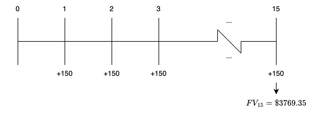
As indicated here, the sum of the compounded values of the individual cash flows in this 15-year ordinary annuity is $3,769.35. Note that the annuity payments themselves amounted to $2,250 = 15 × $150, and the balance is the interest earned at the rate of 7% per year.

To find the PV of an ordinary annuity, we use the future cash flow stream, PMT, that we used with FV annuity problems, but we discount the cash flows back to the present (time = 0) rather than compounding them forward to the terminal date of the annuity.

Here again, the PMT variable is a single periodic payment, not the total of all the payments (or deposits) in the annuity. The PVAO measures the collective PV of a stream of equal cash flows received at the end of each compounding period over a stated number of periods, N, given a specified rate of return, I/Y. The following examples illustrate how to determine the PV of an ordinary annuity using a financial calculator.

Example: PV of an ordinary annuity

What is the PV of an annuity that pays $200 per year at the end of each of the next 13 years given a 6% discount rate?

Answer:

The payments occur at the end of the year, so this annuity is an ordinary annuity. To solve this problem, enter the relevant information and compute PV.

$N = 13; I/Y = 6; PMT = -200; CPT → PV = 1,770.54$

The $1,770.54 computed here represents the amount of money that an investor would need to invest today at a 6% rate of return to generate 13 end-of-year cash flows of $200 each.

Example: PV of an ordinary annuity beginning later than t = 1

What is the present value of four $100 end-of-year payments if the first payment is to be received three years from today and the appropriate rate of return is 9%?

Answer:

The time line for this cash flow stream is shown in the following figure.

PV of an Annuity Beginning at $t = 3$

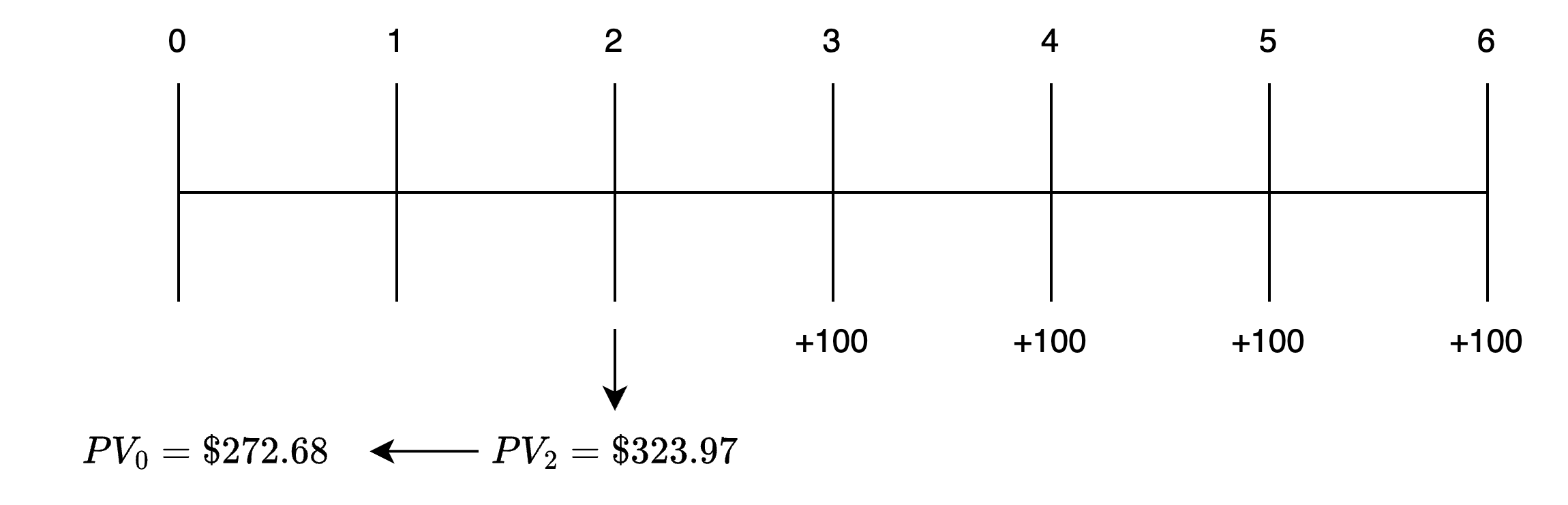
Step 1: Find the present value of the annuity as of the end of year 2 ($PV_{2}$).

Input the relevant data and solve for $PV_{2}$.

$N = 4; I/Y = 9; PMT = -100; CPT → PV = PV_{2} = 323.97$

Step 2: Find the present value of $PV_{2}$.

Input the relevant data and solve for $PV_{0}$.

$N = 2; I/Y = 9; PMT = 0; FV = -323.97; CPT → PV = PV_{0} = 272.68$

In this solution, the annuity was treated as an ordinary annuity. The PV was computed one period before the first payment, and we discounted $PV_{2} =$ $$323.97$ over two years. We need to stress this important point. The PV annuity function on your calculator set in "END" mode gives you the value one period before the annuity begins. Although the annuity begins at $t = 3$, we discounted the result for only two periods to get the present ($t = 0$) value.

Future Value of an Annuity Due

Sometimes it is necessary to find the FV of an annuity due ($FVA_{D}$), an annuity where the annuity payments (or deposits) occur at the beginning of each compounding period. Fortunately, our financial calculators can be used to do this, but with one slight modification—the calculator must be set to the beginning-of-period (BGN) mode. To switch between the BGN and END modes on the TI, press [2nd] [BGN] [2nd] [SET]. When this is done, “BGN” will appear in the upper right corner of the display window. If the display indicates the desired mode, press [2nd] [QUIT]. You will normally want your calculator to be in the ordinary annuity (END) mode, so remember to switch out of BGN mode after working annuity due problems. Note that nothing appears in the upper right corner of the display window when the TI is set to the END mode. It should be mentioned that while annuity due payments are made or received at the beginning of each period, the FV of an annuity due is calculated as of the end of the last period.

Another way to compute the FV of an annuity due is to calculate the FV of an ordinary annuity, and simply multiply the resulting $FV$ by $[1 + \text{periodic compounding rate} (I/Y)]$. Symbolically, this can be expressed as:

$$\text{FVA}_{D} = \text{FVA}_{O} \times (1 + I/Y)$$

The following examples illustrate how to compute the FV of an annuity due.

Example: FV of an annuity due

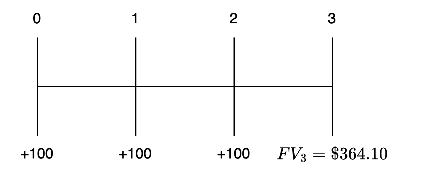
What is the future value of an annuity that pays $100 per year at the beginning of each of the next three years, commencing today, if the cash flows can be invested at an annual rate of 10%? Note in the time line in the figure below that the FV is computed as of the end of the last year in the life of the annuity, year 3, even though the final payment occurs at the beginning of year 3 (end of year 2).

Answer:

To solve this problem, put your calculator in the BGN mode ([2nd] [BGN] [2nd] [SET] [2nd] [QUIT] on the TI or [g] [BEG] on the HP), then input the relevant data and compute FV:

$N = 3, I/Y = 10, PMT = 100, CPT → FV = 364.10$

FV of an Annuity Due

Alternatively, we could calculate the FV for an ordinary annuity and multiply it by $1 + I/Y$. Leaving your calculator in the END mode, enter the following inputs:

$N = 3, I/Y = 10, PMT = 100, CPT → FVA_{0} = 331.00$

$\text{FVA}_D = \text{FVA}_O \times (1 + I/Y) = 331.00 \times 1.10 = 364.10$

Present Value of an Annuity Due

While less common than those for ordinary annuities, some problems may require you to find the PV of an annuity due (PVAD). Using a financial calculator, this really shouldn’t be much of a problem. With an annuity due, there is one less discounting period since the first cash flow occurs at t = 0 and thus is already its PV. This implies that, all else equal, the PV of an annuity due will be greater than the PV of an ordinary annuity.

As you will see in the next example, there are two ways to compute the PV of an annuity due. The first is to put the calculator in the BGN mode and then input all the relevant variables (PMT, I/Y, and N) as you normally would. The second, and far easier way, is to treat the cash flow stream as an ordinary annuity over N compounding periods, and simply multiply the resulting PV by [1 + periodic compounding rate (I/Y)].

Symbolically, this can be stated as:

$$\text{PVA}_D = \text{PVA}_O \times (1 + I/Y)$$

The advantage of this second method is that you leave your calculator in the END mode and won’t run the risk of forgetting to reset it. Regardless of the procedure used, the computed PV is given as of the beginning of the first period, $t = 0$.

Example: PV of an annuity due

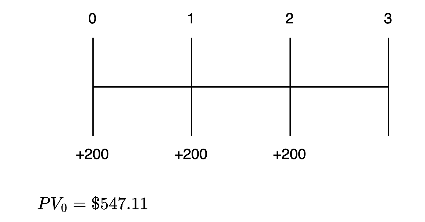
Given a discount rate of 10%, what is the present value of an annuity that makes $200 payments at the beginning of each of the next three years, starting today?

Answer:

First, let’s solve this problem using the calculator’s BGN mode. Set your calculator to the BGN mode ([2nd] [BGN] [2nd] [SET] [2nd] [QUIT] on the TI or [g] [BEG] on the HP), enter the relevant data, and compute PV.

$N = 3; I/Y = 10; PMT = -200; CPT → \text{PVA}_D = 547.11$

The time line for this problem is shown in the following figure.

PV of an Annuity Due

Alternatively, this problem can be solved by leaving your calculator in the END mode. First, compute the PV of an ordinary 3-year annuity. Then multiply this PV by (1 + I/Y). To use this approach, enter the relevant inputs and compute PV.

$N = 3; I/Y = 10; PMT = -200; CPT → \text{PVA}_O = 497.37$

$\text{PVA}_D = \text{PVA}_O \times (1 + I/Y) = 497.37 \times 1.10 = 547.11$

Present Value of a Perpetuity

A perpetuity is a financial instrument that pays a fixed amount of money at set intervals over an infinite period of time. In essence, a perpetuity is a perpetual annuity. Most preferred stocks are examples of perpetuities since they promise fixed interest or dividend payments forever. Without going into all the excruciating mathematical details, the discount factor for a perpetuity is just one divided by the appropriate rate of return (i.e., 1/r). Given this, we can compute the PV of a perpetuity.

$$\text{PV}_{perpetuity} = \frac{PMT}{I/Y}$$

The PV of a perpetuity is the fixed periodic cash flow divided by the appropriate periodic rate of return.

As with other TVM applications, it is possible to solve for unknown variables in the $\text{PV}_{perpetuity}$ equation. In fact, you can solve for any one of the three relevant variables, given the values for the other two.

EXAMPLE: PV of a perpetuity

Kodon Corporation issues preferred stock that will pay $4.50 per year in annual dividends beginning next year and plans to follow this dividend policy forever. Given an 8% rate of return, what is the value of Kodon’s preferred stock today?

Answer: Given that the value of the stock is the PV of all future dividends, we have:

$$PV_{perpetuity} = \frac{4.50}{0.08} = \$56.25$$

Thus, if an investor requires an 8% rate of return, the investor should be willing to pay $56.25 for each share of Kodon’s preferred stock. Note that the PV of a perpetuity is its value one period before its next payment.

EXAMPLE: PV of a deferred perpetuity

Assume the Kodon preferred stock in the preceding examples is scheduled to pay its first dividend in four years, and is non-cumulative (i.e., does not pay any dividends for the first three years). Given an $8% required rate of return, what is the value of Kodon’s preferred stock today?

Answer: As in the previous example,

$$PV_{perpetuity} = \frac{4.50}{0.08} = \$56.25,$$

but because the first dividend is paid at $t = 4$, this PV is the value at $t = 3$ . To get the value of the preferred stock today, we must discount this value for three periods:

$$\frac{56.25}{(1.08)^3} = \$44.65.$$

📝 Quiz

1. The amount an investor will have in 15 years if $1,000 is invested today at an annual interest rate of 9% will be closest to:

• A. $1,350.
• B. $3,518.
• C. $3,642.

2. How much must be invested today, at 8% interest, to accumulate enough to retire a $10,000 debt due seven years from today?

• A. $5,835.
• B. $6,123.
• C. $8,794.

3. An investor has just won the lottery and will receive $50,000 per year at the end of each of the next 20 years. At a 10% interest rate, the present value of the winnings is closest to:

• A. $425,678.
• B. $637,241.
• C. $2,863,750.

4. An investor is to receive a 15-year, $8,000 annuity, with the first payment to be received today. At an 11% discount rate, this annuity's worth today is closest to:

• A. $55,855.
• B. $57,527.
• C. $63,855.

5. If $1,000 is invested today and $1,000 is invested at the beginning of each of the next three years at 12% interest (compounded annually), the amount an investor will have at the end of the fourth year will be closest to:

• A. $4,779.
• B. $5,353.
• C. $6,792.

6. Terry Corporation preferred stocks are expected to pay a $9 annual dividend forever. If the required rate of return on equivalent investments is 11%, a share of Terry preferred should be worth:

• A. $81.82.
• B. $99.00.
• C. $122.22.

Uneven Cash Flows

It is not uncommon to have applications in investments and corporate finance where it is necessary to evaluate a cash flow stream that is not equal from period to period. The time line in Figure depicts such a cash flow stream.

Figure: Time Line for Uneven Cash Flows

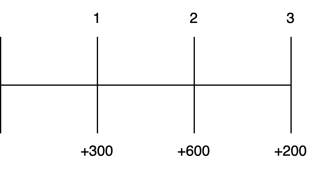
This three-year cash flow series is not an annuity since the cash flows are different every year. In essence, this series of uneven cash flows is nothing more than a stream of annual single sum cash flows. Thus, to find the PV or FV of this cash flow stream, all we need to do is sum the PVs or FVs of the individual cash flows.

EXAMPLE: Computing the FV of an uneven cash flow series

Using a rate of return of 10%, compute the future value of the three-year uneven cash flow stream described above at the end of the third year.

Answer:

The FV for the cash flow stream is determined by first computing the FV of each individual cash flow, then summing the FVs of the individual cash flows.

$$FV_1: PV = -300; I/Y = 10; N = 2; CPT \rightarrow FV = FV_1 = 363$$ $$FV_2: PV = -600; I/Y = 10; N = 1; CPT \rightarrow FV = FV_2 = 660$$ $$FV_3: PV = -200; I/Y = 10; N = 0; CPT \rightarrow FV = FV_3 = 200$$ $$FV \text{ of cash flow stream} = \Sigma FV_{\text{individual}} = 1,223$$

EXAMPLE: Computing PV of an uneven cash flow series

Compute the present value of this three-year uneven cash flow stream described previously using a 10% rate of return.

Answer:

This problem is solved by first computing the PV of each individual cash flow, then summing the PVs of the individual cash flows, which yields the PV of the cash flow stream. Again the signs of the cash flows are preserved.

$$PV_1: FV = 300; I/Y = 10; N = 1; CPT \rightarrow PV = PV_1 = -272.73$$ $$PV_2: FV = 600; I/Y = 10; N = 2; CPT \rightarrow PV = PV_2 = -495.87$$ $$PV_3: FV = 200; I/Y = 10; N = 3; CPT \rightarrow PV = PV_3 = -150.26$$ $$PV \text{ of cash flow stream} = \sum PV_{\text{individual}} = \$918.86$$

Solving Time Value of Money Problems When Compounding Periods Are Other Than Annual

While the conceptual foundations of TVM calculations are not affected by the compounding period, more frequent compounding does have an impact on FV and PV computations. Specifically, since an increase in the frequency of compounding increases the effective rate of interest, it also increases the FV of a given cash flow and decreases the PV of a given cash flow.

EXAMPLE: The effect of compounding frequency on FV and PV

Compute the FV one year fr om now of $1,000 today and the PV of $1,000 to be received one year from now using a stated annual interest rateF of 6% with a range of compounding periods.

Answer: Compounding Frequency Effect

$$\begin{array}{|l|c|c|c|c|} \hline \text{Compounding Frequency} & \text{Interest Rate per Period} & \text{Effective Annual Rate} & \text{Future Value} & \text{Present Value} \\ \hline \text{Annual (m = 1)} & 6.000\% & 6.00\% & \$1,060.00 & \$943.396 \\ \text{Semiannual (m = 2)} & 3.000 & 6.090 & 1,060.90 & 942.596 \\ \text{Quarterly (m = 4)} & 1.500 & 6.136 & 1,061.36 & 942.184 \\ \text{Monthly (m = 12)} & 0.500 & 6.168 & 1,061.68 & 941.905 \\ \text{Daily (m = 365)} & 0.016438 & 6.183 & 1,061.83 & 941.769 \\ \hline \end{array}$$

There are two ways to use your financial calculator to compute PVs and FVs under different compounding frequencies:

1. Adjust the number of periods per year (P/Y) mode on your calculator to correspond to the compounding frequency (e.g., for quarterly, P/Y = 4). WE DO NOT RECOMMEND THIS APPROACH!
2. Keep the calculator in the annual compounding mode (P/Y = 1) and enter I/Y as the interest rate per compounding period, and N as the number of compounding periods in the investment horizon. Letting m equal the number of compounding periods per year, the basic formulas for the calculator input data are determined as follows:

$$I/Y = \text{the annual interest rate} / m$$ $$N = \text{the number of years} × m$$

The computations for the FV and PV amounts in the previous example are:

$$PV_A: FV = -1,000; I/Y = 6 / 1 = 6; N = 1 × 1 = 1: CPT → PV = PV_A = 943.396$$ $$PV_S: FV = -1,000; I/Y = 6 / 2 = 3; N = 1 × 2 = 2: CPT → PV = PV_S = 942.596$$ $$PV_Q: FV = -1,000; I/Y = 6 / 4 = 1.5; N = 1 × 4 = 4: CPT → PV = PV_Q = 942.184$$ $$PV_M: FV = -1,000; I/Y = 6 / 12 = 0.5; N = 1 × 12 = 12: CPT → PV = PV_M = 941.905$$ $$PV_D: FV = -1,000; I/Y = 6 / 365 = 0.016438; N = 1 × 365 = 365: CPT → PV = PV_D = 941.769$$ $$FV_A: PV = -1,000; I/Y = 6 / 1 = 6; N = 1 × 1 = 1: CPT → FV = FV_A = 1,060.00$$ $$FV_S: PV = -1,000; I/Y = 6 / 2 = 3; N = 1 × 2 = 2: CPT → FV = FV_S = 1,060.90$$ $$FV_Q: PV = -1,000; I/Y = 6 / 4 = 1.5; N = 1 × 4 = 4: CPT → FV = FV_Q = 1,061.36$$ $$FV_M: PV = -1,000; I/Y = 6 / 12 = 0.5; N = 1 × 12 = 12: CPT → FV = FV_M = 1,061.68$$ $$FV_D: PV = -1,000; I/Y = 6 / 365 = 0.016438; N = 1 × 365 = 365: CPT → FV = FV_D = 1,061.83$$

EXAMPLE: FV of a single sum using quarterly compounding

Compute the FV of $2,000 today, five years from today using an interest rate of 12%, compounded quarterly.

Answer:

To solve this problem, enter the relevant data and compute FV:

$$N = 5 × 4 = 20; I/Y = 12 / 4 = 3; PV = -\$2,000; CPT → FV = \$3,612.22$$

E. Demonstrate the use of a time line in modeling and solving time value of money problems.

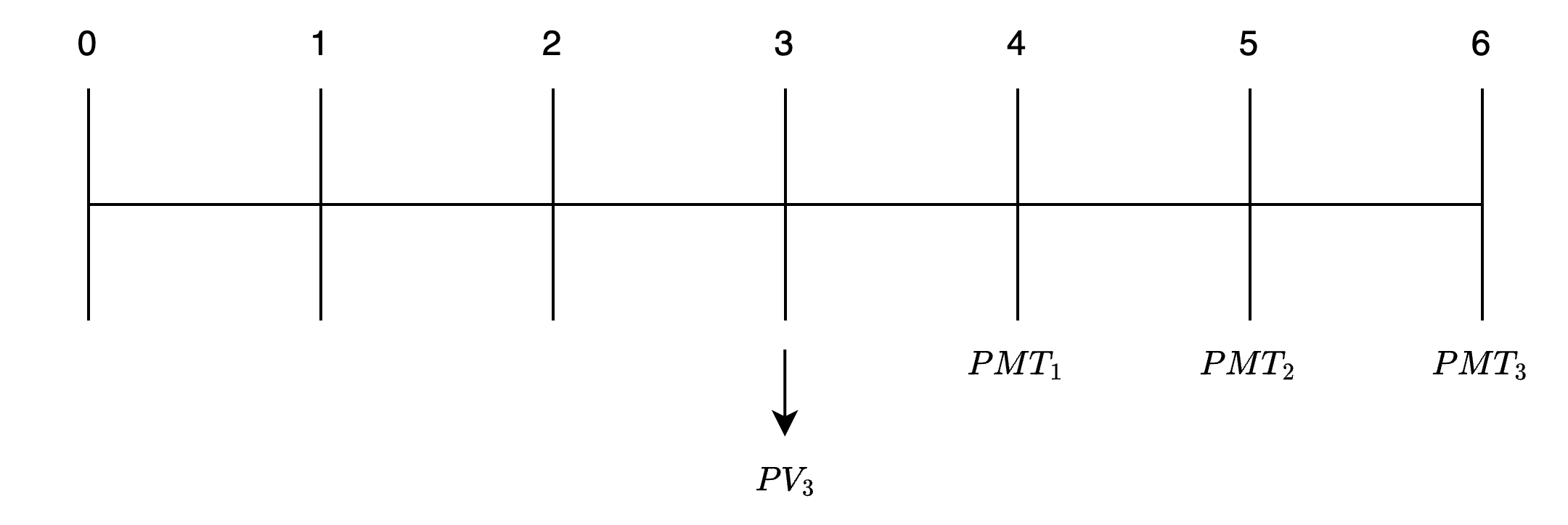
In most of the PV problems we have discussed, cash flows were discounted back to the current period. In this case, the PV is said to be indexed to t = 0, or the time index is t = 0. For example, the PV of a 3-year ordinary annuity that is indexed to t = 0 is computed at the beginning of Year 1 (t = 0). Contrast this situation with another 3-year ordinary annuity that doesn’t start until Year 4 and extends to Year 6. It would not be uncommon to want to know the PV of this annuity at the beginning of Year 4, in which case the time index is t = 3. The time line for this annuity is presented in the following Figure.

Figure: Indexing Time Line to Other Than t = 0

The following examples will illustrate how to compute I/Y, N, or PMT in annuity problems.

Example: Computing an annuity payment needed to achieve a given FV

At an expected rate of return of 7%, how much must be deposited at the end of each year for the next 15 years to accumulate $3,000?

Answer:

To solve this problem, enter the three relevant known values and compute PMT.

$$N = 15; I/Y = 7; FV = +\$3,000; CPT → PMT = –\$119.38 \ \text{(ignore sign)}$$

EXAMPLE: Computing a loan payment

Suppose you are considering applying for a $2,000 loan that will be repaid with equal end-of-year payments over the next 13 years. If the annual interest rate for the loan is 6%, how much will your payments be?

Answer:

The size of the end-of-year loan payment can be determined by inputting values for the three known variables and computing PMT.

$$N = 13; I/Y = 6; PV = –2,000; CPT → PMT = \$225.92$$

EXAMPLE: Computing the number of periods in an annuity

How many $100 end-of-year payments are required to accumulate $920 if the discount rate is 9%?

Answer:

The number of payments necessary can be determined by inputting the relevant data and computing N.

$$I/Y = 9\%; FV = \$920; PMT = –\$100; CPT → N = 7 \ \text{years}$$

It will take seven annual $100 payments, compounded at 9% annually, to accrue an investment value of $920.

PROFESSOR’S NOTE

Remember the sign convention. PMT and FV must have opposite signs or your calculator will issue an error message.

EXAMPLE: Computing the number of years in an ordinary annuity

Suppose you have a $1,000 ordinary annuity earning an 8% return. How many annual end-of-year $150 withdrawals can be made?

Answer:

The number of years in the annuity can be determined by entering the three relevant variables and computing N.

$$I/Y = 8; PMT = 150; PV = –1,000; CPT → N = 9.9 \ \text{years}$$

EXAMPLE: Computing the rate of return for an annuity

Suppose you have the opportunity to invest $100 at the end of each of the next five years in exchange for $600 at the end of the fifth year. What is the annual rate of return on this investment?

Answer:

The rate of return on this investment can be determined by entering the relevant data and solving for I/Y.

$$N = 5; FV = \$600; PMT = –100; CPT → I/Y = 9.13\%$$

EXAMPLE: Computing the discount rate for an annuity

What rate of return will you earn on an ordinary annuity that requires a $700 deposit today and promises to pay $100 per year at the end of each of the next 10 years?

Answer:

The discount rate on this annuity is determined by entering the three known values and computing I/Y.

$$N = 10; PV = –700; PMT = 100; CPT → I/Y = 7.07\%$$

Funding a Future Obligation

There are many TVM applications where it is necessary to determine the size of the deposit(s) that must be made over a specified period in order to meet a future liability, such as setting up a funding program for future college tuition or a retirement program. In most of these applications, the objective is to determine the size of the payment(s) or deposit(s) necessary to meet a particular monetary goal.

EXAMPLE: Computing the required payment to fund an annuity due

Suppose you must make five annual $1,000 payments, the first one starting at the beginning of Year 4 (end of Year 3). To accumulate the money to make these payments, you want to make three equal payments into an investment account, the first to be made one year from today. Assuming a 10% rate of return, what is the amount of these three payments?

Answer:

The time line for this annuity problem is shown in the following figure.

Funding an Annuity Due

The first step in this type of problem is to determine the amount of money that must be available at the beginning of Year 4 (t = 3) in order to satisfy the payment requirements. This amount is the PV of a 5-year annuity due at the beginning of Year 4 (end of Year 3). To determine this amount, set your calculator to the BGN mode, enter the relevant data, and compute PV.

$$N = 5; I/Y = 10; PMT = -1,000; CPT → PV = PV_{3} = \$4,169.87$$

Alternatively, you can leave your calculator in the END mode, compute the PV of a 5-year ordinary annuity, and multiply by 1.10.

$$N = 5; I/Y = 10; PMT = -1,000; CPT → PV = 3,790.79 × 1.1 = PV_{3} = \$4,169.87$$

A third alternative, with the calculator in END mode, is to calculate the t = 3 value of the last four annuity payments and then add $1,000.

$$N = 4; I/Y = 10; PMT = -1,000; CPT → PV = 3,169.87 + 1,000 = \$4,169.87 = PV_{3}$$

$PV_{3}$ becomes the FV that you need three years from today from your three equal end-of-year deposits. To determine the amount of the three payments necessary to meet this funding requirement, be sure that your calculator is in the END mode, input the relevant data, and compute PMT.

$$N = 3; I/Y = 10; FV = -4,169.87; CPT → PMT = \$1,259.78$$

The second part of this problem is an ordinary annuity. If you changed your calculator to BGN mode and failed to put it back in the END mode, you will get a PMT of $1,145, which is incorrect.

The Connection Between Present Values, Future Values, and Series of Cash Flows

As we have explained in the discussion of annuities and series of uneven cash flows, the sum of the present values of the cash flows is the present value of the series. The sum of the future values (at some future time = n) of a series of cash flows is the future value of that series of cash flows.

One interpretation of the present value of a series of cash flows is how much would have to be put in the bank today in order to make these future withdrawals and exhaust the account with the final withdrawal. Let’s illustrate this with cash flows of $100 in Year 1, $200 in Year 2, $300 in Year 3, and an assumed interest rate of 10%.

Calculate the present value of these three cash flows as:

$$\frac{100}{1.1} + \frac{200}{1.1^2} + \frac{300}{1.1^3} = \$481.59$$

If we put $481.59 in an account yielding 10%, at the end of the year we would have 481.59 × 1.1 = $529.75. Withdrawing $100 would leave $429.75.

Over the second year, the $429.75 would grow to 429.75 × 1.1 = $472.73. Withdrawing $200 would leave $272.73.

Over the third year, $272.73 would grow to 272.73 × 1.1 = $300, so that the last withdrawal of $300 would empty the account.

The interpretation of the future value of a series of cash flows is straightforward as well. The FV answers the question, “How much would be in an account when the last of a series of deposits is made?” Using the same three cash flows—$100, $200, and $300—and the same interest rate of 10%, we can calculate the future value of the series as:

$$100(1.1)^2 + 200(1.1) + 300 = \$641$$

This is simply the sum of the t = 3 value of each of the cash flows. Note that the t = 3 value and the t = 0 (present) value of the series are related by the interest rate, $481.59(1.1)^3 = 641$.

The $100 cash flow (deposit) comes at t = 1, so it will earn interest of 10% compounded for two periods (until t = 3). The $200 cash flow (deposit) will earn 10% between t = 2 and t = 3, and the final cash flow (deposit) of $300 is made at t = 3, so $300 is the future (t = 3) value of that cash flow.

We can also look at the future value in terms of how the account grows over time. At t = 1 we deposit $100, so at t = 2 it has grown to $110 and the $200 deposit at t = 2 makes the account balance $310. Over the next period, the $310 grows to 310 × 1.1 = $341 at t = 3, and the addition of the final $300 deposit puts the account balance at $641. This is, of course, the future value we calculated initially.

PROFESSOR’S NOTE

This last view of the future value of a series of cash flows suggests a quick way to calculate the future value of an uneven cash flow series. The process described previously for the future value of a series of end-of-period payments can be written mathematically as [(100 × 1.1) + 200] × 1.1 + 300 = 641, and this might be a quick way to do some future value problems.

Note that questions on the future value of an annuity due refer to the amount in the account one period after the last deposit is made. If the three deposits considered here were made at the beginning of each period (at t = 0, 1, 2) the amount in the account at the end of three years (t = 3) would be 10% higher (i.e., 641 × 1.1 = $705.10).

The cash flow additivity principle refers to the fact that present value of any stream of cash flows equals the sum of the present values of the cash flows. There are different applications of this principle in time value of money problems. If we have two series of cash flows, the sum of the present values of the two series is the same as the present values of the two series taken together, adding cash flows that will be paid at the same point in time. We can also divide up a series of cash flows any way we like, and the present value of the “pieces” will equal the present value of the original series.

EXAMPLE: Additivity principle

A security will make the following payments at the end of the next four years: $100, $100, $400, and $100. Calculate the present value of these cash flows using the concept of the present value of an annuity when the appropriate discount rate is 10%.

Answer:

We can divide the cash flows so that we have:

t = 1	t = 2	t = 3	t = 4
100	100	100	100	cash flow series #1
0	0	300	0	cash flow series #2
------	-------	-------	-------
$100	$100	$400	$100

The additivity principle tells us that to get the present value of the original series, we can just add the present values of series #1 (a 4-period annuity) and series #2 (a single payment three periods from now).

For the annuity: $N = 4; PMT = 100; FV = 0; I/Y = 10; CPT → PV = -\$316.99$

For the single payment: $N = 3; PMT = 0; FV = 300; I/Y = 10; CPT → PV = -\$225.39$

The sum of these two values is $316.99 + 225.39 = \$542.38$.

The sum of these two (present) values is identical (except for rounding) to the sum of the present values of the payments of the original series:

$$\frac{100}{1.1} + \frac{100}{1.1^2} + \frac{400}{1.1^3} + \frac{100}{1.1^4} = \$542.38$$

📝 Quiz

1. An analyst estimates that XYZ’s earnings will grow from $3.00 a share to $4.50 per share over the next eight years. The rate of growth in XYZ’s earnings is closest to:

• A. 4.9%.
• B. 5.2%.
• C. 6.7%.

2. If $5,000 is invested in a fund offering a rate of return of 12% per year, approximately how many years will it take for the investment to reach $10,000?

• A. 4 years.
• B. 5 years.
• C. 6 years.

3. An investment is expected to produce the cash flows of $500, $200, and $800 at the end of the next three years. If the required rate of return is 12%, the present value of this investment is closest to:

• A. $835.
• B. $1,175.
• C. $1,235.

4. If $10,000 is invested today in an account that earns interest at a rate of 9.5%, what is the value of the equal withdrawals that can be taken out of the account at the end of each of the next five years if the investor plans to deplete the account at the end of the time period?

• A. $2,453.
• B. $2,604.
• C. $2,750.

5. Given an 11% rate of return, the amount that must be put into an investment account at the end of each of the next 10 years in order to accumulate $60,000 to pay for a child’s education is closest to:

• A. $2,500.
• B. $3,588.
• C. $4,432.

6. An investor will receive an annuity of $4,000 a year for 10 years. The first payment is to be received five years from today. At a 9% discount rate, this annuity’s worth today is closest to:

• A. $16,684.
• B. $18,186.
• C. $25,671.

7. An investor is looking at a $150,000 home. If 20% must be put down and the balance is financed at 9% over the next 30 years, what is the monthly mortgage payment?

• A. $799.33.
• B. $895.21.
• C. $965.55.

References

• https://youssef-serghini.weebly.com/5-the-time-value-of-money.html